Detect Lines Using Radon Transform

R2026b

This example shows how to use the Radon transform to detect lines in an image. The Radon transform is closely related to a common computer vision operation known as the Hough transform. You can use the radon function to implement a form of the Hough transform used to detect straight lines.

Calculate the Radon Transform of an Image

Read and display a grayscale image.

I = fitsread("solarspectra.fts");
I = rescale(I);
imshow(I)
title("Original Image")

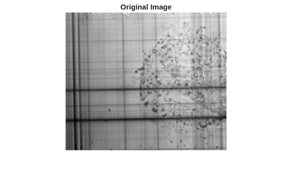
Find the edges within the image by using the edge function, then display the resulting binary image.

BW = edge(I);
imshow(BW)
title("Edges of Original Image")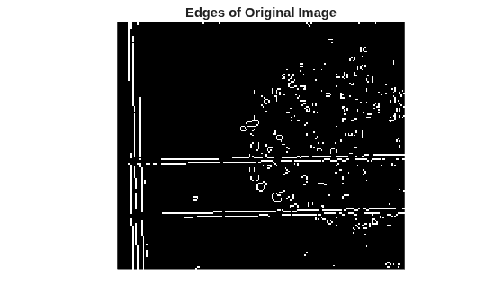

Calculate the Radon transform of the binary image by using the radon function.

theta = 0:179;
[R,xp] = radon(BW,theta);

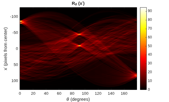
Display the result of the Radon transform. Peaks in the transform indicate straight lines in the original image.

imagesc(theta,xp,R)
colormap(hot)
xlabel("\theta (degrees)")
ylabel("x^{\prime} (pixels from center)")
title("R_{\theta} (x^{\prime})")
colorbar

Interpret the Peaks of the Radon Transform

Find the indices of the largest peaks by using the maxk function, then convert the indices to row and column coordinates by using the ind2sub function.

numPeaks = 5;
[~,idxPeaks] = maxk(R(:),numPeaks);
[rowPeaks,colPeaks] = ind2sub(size(R),idxPeaks);

Determine the projection angles, θ, for peaks in the Radon transform, by finding the values of the theta variable at the indices specified by colPeaks.

thetaPeaks = theta(colPeaks)

thetaPeaks = 1×5

     1    91     1     1    91

Determine the offsets, x', for peaks in the Radon transform, by finding the values of the xp variable at the indices specified by rowPeaks. The offsets are of the lines from the center of the image, in pixels.

xpPeaks = xp(rowPeaks)'

xpPeaks = 1×5

   -80   -44   -84   -87    -8

Inspect the values of the thetaPeaks and xpPeaks vectors. The strongest peak (represented by the first element in each vector) corresponds to a line with a projection angle of θ = 1 degree and an offset of x' = –80 pixels from center. Two of the remaining strongest peaks represent lines that are parallel to the strongest peak (θ = 1) with different offsets (–84 pixels and –87 pixels). The other two strongest peaks represent a pair of parallel lines with θ = 91 degrees and offsets of –44 pixels and –8 pixels from center.

Represent Lines in Cartesian Coordinates

The projection angles in the Radon transform are perpendicular to the corresponding lines in the original image. Calculate the angles of the lines corresponding to the largest peaks.

thetaLines = thetaPeaks+90;

Convert the angles of the projections and image lines from degrees to radians.

thetaPeaksRadians = deg2rad(thetaPeaks);
thetaLinesRadians = deg2rad(thetaLines);

Convert the projections and image lines from polar coordinates to Cartesian coordinates by using the pol2cart function. The pol2cart function returns x- and y-coordinates of the endpoints of lines of length rho. Specify a value of rho that is half of the larger dimension of the image.

centerX = ceil(size(I,2)/2);
centerY = ceil(size(I,1)/2);
rho = max(centerX,centerY);
[xsPeaks,ysPeaks] = pol2cart(thetaPeaksRadians,rho);
[xsLines,ysLines] = pol2cart(thetaLinesRadians,rho);

Shift the lines from the origin to the center of the image. In Image Processing Toolbox, the origin is at the top left not bottom left, so reverse the y-coordinates of the endpoints.

xLims = [-xsLines; xsLines] + centerX;
yLims = [ysLines; -ysLines] + centerY;

Apply the offset to the lines, reversing the direction of the offset in the y direction.

xLims = xLims + xpPeaks.*cosd(thetaPeaks);  
yLims = yLims - xpPeaks.*sind(thetaPeaks);  

Display Peak Projection and Corresponding Line

To visualize the relationship between the Radon transform and lines in the image, annotate the original image to highlight one of the projections and the corresponding line in the image.

First, display a copy of the original image and mark the center of the image with a blue x symbol.

figure
hold on
imshow(I)
scatter(centerX,centerY,"bx",LineWidth=2)

Select a projection and get the x- and y-coordinates of the endpoints of the projection. Then, draw the projection as a green dashed line. The projection goes through the center of the image.

peakID = 3;
xLimsPeak = [centerX-xsPeaks(peakID) centerX+xsPeaks(peakID)];
yLimsPeak = [centerY+ysPeaks(peakID) centerY-ysPeaks(peakID)];
plot(xLimsPeak,yLimsPeak,"g--",LineWidth=2)

Draw the perpendicular to the projection as a red dashed line. The perpendicular has the same angle as the line in the image, but omits the offset.

xLimsPerp = [centerX-xsLines(peakID) centerX+xsLines(peakID)];
yLimsPerp = [centerY+ysLines(peakID) centerY-ysLines(peakID)];
plot(xLimsPerp,yLimsPerp,"r--",LineWidth=2)

Draw the actual line in the image, including the offset, as a solid red line.

plot(xLims(:,peakID),yLims(:,peakID),"r",LineWidth=2)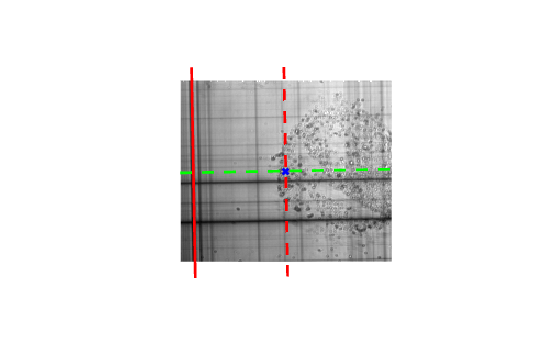

Display Lines in Order of Strength

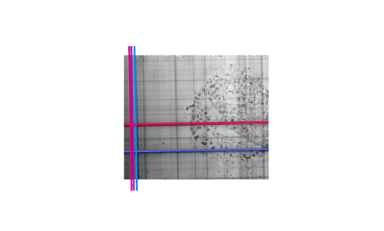
Draw all of the strongest lines on the image. Indicate the order of strength by using the nebula colormap. The colors of the lines change from blue to purple to pink in order of decreasing line strength.

figure
hold on
imshow(I)
p = plot(xLims,yLims,LineWidth=2);
set(p,{"Color"},num2cell(nebula(numPeaks),2))