Create an App for Soil Mapping Using Hyperspectral Imagery

R2026b

Since R2026b

This example shows how to build an interactive app for generating soil property maps from hyperspectral image data. The soilMappingApp app enables you to load hyperspectral data, preprocess it, mask non-soil regions such as water and vegetation, compute spectral soil indices, and export the results for further analysis.

Soil mapping from remote sensing data uses spectral signatures to identify and quantify soil properties such as organic matter content, clay minerals, iron oxides, and soil moisture. This approach builds on techniques developed for hyperspectral soil analysis, where spectral indices derived from specific wavelength bands serve as indicators of soil composition. The app you build in this example provides a set of spectral index algorithms that you can apply interactively to hyperspectral imagery to produce soil parameter maps.

The soilMappingApp app is also attached to this example as supporting files. To directly run the app, see the Run the Soil Mapping App section.

Create the App Window and Panel Layout

The soilMappingApp app has three main panels.

1. Soil Mapping Tools (left panel) — Contains controls for loading data, preprocessing, masking, index selection, and export.

2. Image and Index Viewer (center panel) — Displays the hyperspectral image and computed soil index maps using a viewer2d object with overlay support.

3. Info (right panel) — Shows image metadata, a histogram of the computed index, and thresholding controls.

The app uses a programmatic UI approach with uifigure and uigridlayout to create a responsive layout.

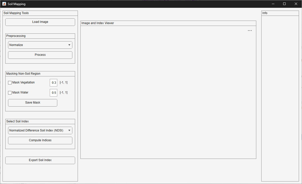
The main function soilMappingApp creates a uifigure window and arranges the three panels.

fig = uifigure("Name", "Soil Mapping", "Position", [100 100 1200 700]);

The left panel uses a grid layout to stack controls vertically.

% Left Panel
panelLeft = uipanel(fig, "Title", "Soil Mapping Tools", ...
    "Position", [10 10 300 680]);
gridLeft = uigridlayout(panelLeft, [12, 1]);
gridLeft.RowHeight = {30, 10, 120, 10, 160, 10, 120, 10, 30};
gridLeft.ColumnWidth = {'1x'};

The center panel hosts a viewer2d component for image display.

% Center Panel (Viewer)
panelCenter = uipanel(fig, "Title", "Image and Index Viewer", ...
    "Position", [320 100 700 550]);

The right panel holds metadata and analysis tools.

% Right Panel (Info)
panelRight = uipanel(fig, "Title", "Info", ...
    "Position", [1040 10 150 680]);

Load Hyperspectral Data

The app loads hyperspectral data from the workspace. The loadImageFromWorkspace helper function scans the base workspace for hypercube or multicube objects and presents them in a selection dialog. After the user selects a variable, the function generates an RGB preview using the colorize function and displays the image in the viewer2d component. The function also extracts and displays available metadata. The helper function is attached to this example as a supporting file.

function loadImageFromWorkspace(fig)
    % Get all variables from base workspace
    vars = evalin('base', 'whos');
    
    % Filter only multicube or hypercube objects
    isCube = @(v) ismember(v.class, ["hyper.io.multicube", "hyper.io.hypercube"]);
    cubeVars = vars(arrayfun(isCube, vars));
    
    if isempty(cubeVars)
        uialert(fig, "No multicube or hypercube found in workspace.", "No Valid Data");
        return;
    end
    
    % Create temporary figure with uitable to let user select
    selectFig = uifigure("Name", "Select Spectral Image", "Position", [500 500 400 300]);
    uit = uitable(selectFig, ...
        "Data", {cubeVars.name}', ...
        "ColumnName", "Variable Name", ...
        "Position", [20 60 360 200], ...
        "Tag", "cubeTable", ...
        "ColumnEditable", false);
    
    % OK button
    uibutton(selectFig, ...
        "Text", "Load", ...
        "Position", [150 20 100 30], ...
        "ButtonPushedFcn", @(btn, event) loadSelectedCube(selectFig, fig));
end

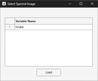
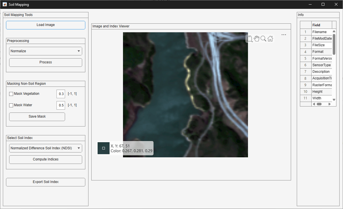
When the user selects a variable and selects Load, the app generates an RGB composite and displays it. The app stores the data cube in the UserData property of the figure for use by other functions.

Preprocess the Hyperspectral Data

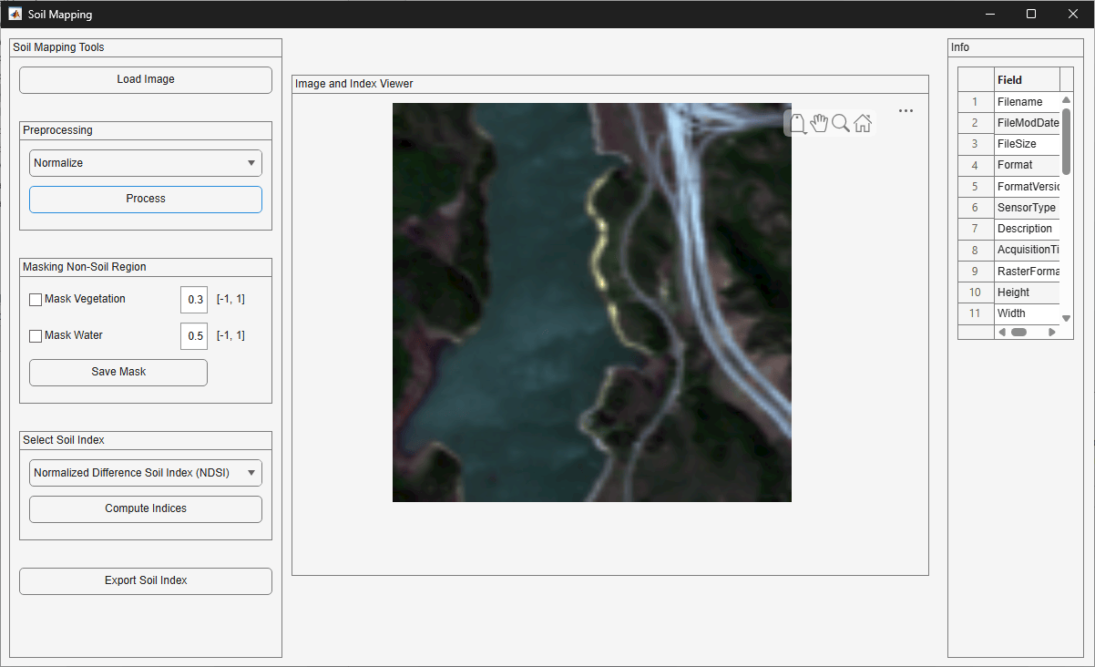
Hyperspectral data often requires preprocessing to convert raw digital numbers into physically meaningful reflectance values. The app provides three preprocessing options through a dropdown menu.

• Normalize — Rescales each band to the [0, 1] range using the rescale function.

• DN to reflectance — Converts digital number (DN) values to reflectance using the dn2reflectance function.

• Atmospheric correction — Applies the simple heuristic atmospheric reflectance correction (SHARC) algorithm using the sharc function.

The applyPreprocessing helper function retrieves the selected method from the dropdown and applies it to the stored data cube. The helper function is attached to this example as a supporting file.

function applyPreprocessing(fig)
    if ~isfield(fig.UserData, "Cube")
        uialert(fig, "Please load an image first.", "No Image");
        return;
    end
    cube = fig.UserData.Cube;
    
    dd = findobj(fig, 'Tag', 'preprocessDropdown');
    selectedAlgo = dd.Value;
    
    try
        switch selectedAlgo
            case "Normalize"
                cube = normalizeCube(cube);
    
            case "DN to reflectance"
                cube = dn2reflectance(cube);
    
            case "Atmospheric correction"
                cube = sharc(cube);
    
            otherwise
                uialert(fig, ...
                    "Unknown pre-processing algorithm selected.", ...
                    "Error", ...
                    "Icon", "error");
                return;
        end
    
    catch ME
        % Catch any error from the selected algorithm
        uialert(fig, ...
            sprintf("An error occurred while running '%s':\n\n%s", selectedAlgo, ME.message), ...
            "Pre-processing Error", ...
            "Icon", "error");
        return;
    end
    fig.UserData.Cube = cube;
    uialert(fig, "Pre-processing Done.",...
        "Preprocessing Complete","Icon","success");
end

Mask Non-Soil Regions

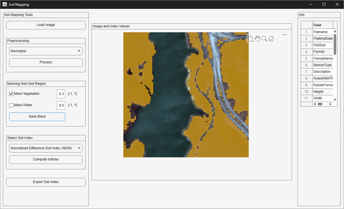
Before computing soil indices, you can mask vegetation and water regions to ensure the analysis focuses exclusively on exposed soil. The masking panel provides checkboxes for vegetation and water, each with an adjustable threshold value in the range [-1, 1].

Vegetation masking uses the normalized difference vegetation index (NDVI), which highlights photosynthetically active surfaces. Water masking uses the modified normalized difference water index (MNDWI), which identifies water bodies. The computeWaterVegMask helper function computes these indices using the spectralIndices function and creates a combined mask based on the selected thresholds. The helper function is attached to this example as a supporting file.

function computeWaterVegMask(fig)
    if ~isfield(fig.UserData, "Cube")
        uialert(fig, "Please load an image first.", "No Image");
        return;
    end
    cube = fig.UserData.Cube;
    
    % Checkboxes
    maskVeg = findobj(fig, 'Tag', 'maskVeg').Value;
    maskWater = findobj(fig, 'Tag', 'maskWater').Value;
    
    % Get checkbox states
    vegBox = findobj(fig, 'Tag', 'vegThresholdBox');
    waterBox = findobj(fig, 'Tag', 'waterThresholdBox');
    
    vegThreshold = vegBox.Value;
    waterThreshold = waterBox.Value;
    
    
    row = size(fig.UserData.Viewer.Children.Data,1);
    col = size(fig.UserData.Viewer.Children.Data,2);
    combinedMask = zeros(row,col);
    
    try
        if maskVeg
            indices = spectralIndices(cube, "NDVI");
            NDVI = indices.IndexImage;
            vegMask = NDVI > vegThreshold;
            combinedMask(vegMask) = 2;  % 2 = vegetation
        end
    
        if maskWater
            indices = spectralIndices(cube, "MNDWI");
            NDWI = indices.IndexImage;
            waterMask = NDWI > waterThreshold;
            % Water overrides only if not already marked as vegetation
            combinedMask(waterMask & combinedMask == 0) = 1;  % 1 = water
        end
    
    catch ME
        % Display a non-blocking alert dialog in the app
        uialert(fig, ...
            sprintf("An error occurred while computing indices:\n\n%s", ME.message), ...
            "Index Computation Error", ...
            "Icon", "error");
        return;
    end
    
    fig.UserData.Mask = combinedMask;
    
    % Display (overlay index map)
    ax = fig.UserData.Viewer;
    ax.CurrentObject.OverlayData = combinedMask;
    
    uialert(fig, "Mask computed and stored. It will be applied during index estimation.",...
        "Masking Complete","Icon","success");
end

The app stores the mask and applies it during soil index computation. Masked pixels appear as NaN values in the output index map.

Compute Soil Indices

The core functionality of the app is computing spectral soil indices that indicate specific soil properties. Each index uses reflectance values at particular wavelengths to characterize a soil attribute. The app supports these indices.

• Normalized Difference Soil Index (NDSI) — Uses bands at 850 nm and 1650 nm to distinguish bare soil from other surfaces.

• Bare Soil Index — Combines four bands (480, 660, 850, and 1650 nm) to identify exposed soil areas.

• Clay Index — Uses the ratio of reflectance at 2200 nm to 2100 nm to detect clay mineral absorption features.

• Organic Matter Index (OMI) — Applies a log-inverse transform to the 1650 nm band to estimate organic carbon content.

• Iron Oxide Index — Uses the ratio of 560 nm to 670 nm reflectance to detect iron oxide minerals.

• Custom Spectral Index — Enables you to define a custom band ratio or normalized difference by specifying wavelengths and a function handle.

The computeIndices helper function selects bands closest to the target wavelengths using a tolerance of 40 nm. This flexibility accommodates sensors with varying spectral resolutions. The helper function is attached to this example as a supporting file.

switch selectedIndex
    case "Normalized Difference Soil Index (NDSI)"
        ind850 = getBandIndex(cube, 850);
        if isempty(ind850)
            showMissingWavelengthAlert(fig, selectedIndex, 850);
        end
        R850 = single(gather(selectBands(cube,'BandNumber',ind850)));
        ind1650 = getBandIndex(cube, 1650);
        if isempty(ind1650)
            showMissingWavelengthAlert(fig, selectedIndex, 1650);
            return;
        end
        R1650 = single(gather(selectBands(cube,'BandNumber',ind1650)));
        idxMap = (R850-R1650)./(R850+R1650+eps);
    case "Clay Index"
        ind2200 = getBandIndex(cube, 2200);
        if isempty(ind2200)
            showMissingWavelengthAlert(fig, selectedIndex, 2200);
            return;
        end
        R2200 = single(gather(selectBands(cube,'BandNumber',ind2200)));
        ind2100 = getBandIndex(cube, 2100);
        if isempty(ind2100)
            showMissingWavelengthAlert(fig, selectedIndex, 2100);
            return;
        end
        R2100 = single(gather(selectBands(cube, 'BandNumber', ind2100)));
        idxMap = R2200./(R2100+eps);
    case "Organic Matter Index (OMI)"
        ind1650 = getBandIndex(cube, 1650);
        if isempty(ind1650)
            showMissingWavelengthAlert(fig, selectedIndex, 1650);
            return;
        end
        R1650 = single(gather(selectBands(cube,'BandNumber',ind1650)));
        idxMap = log10(1./(abs(R1650)+eps));
    case "Iron Oxide Index"
        ind560 = getBandIndex(cube, 560);
        if isempty(ind560)
            showMissingWavelengthAlert(fig, selectedIndex, 560);
            return;
        end
        R560 = single(gather(selectBands(cube, 'BandNumber', ind560)));
        ind670 = getBandIndex(cube, 670);
        if isempty(ind670)
            showMissingWavelengthAlert(fig, selectedIndex, 670);
            return;
        end
        R670 = single(gather(selectBands(cube, 'BandNumber', ind670)));
        idxMap = R560./(R670+eps);
    case "Bare Soil Index"
        ind1650 = getBandIndex(cube, 1650);
        if isempty(ind1650)
            showMissingWavelengthAlert(fig, selectedIndex, 1650);
            return;
        end
        R1650 = single(gather(selectBands(cube, 'BandNumber', ind1650)));
        ind660 = getBandIndex(cube, 660);
        if isempty(ind660)
            showMissingWavelengthAlert(fig, selectedIndex, 660);
            return;
        end
        R660 = single(gather(selectBands(cube, 'BandNumber', ind660)));
        ind850 = getBandIndex(cube, 850);
        if isempty(ind850)
            showMissingWavelengthAlert(fig, selectedIndex, 850);
            return;
        end
        R850 = single(gather(selectBands(cube, 'BandNumber', ind850)));
        ind480 = getBandIndex(cube, 480);
        if isempty(ind480)
            showMissingWavelengthAlert(fig, selectedIndex, 480);
            return;
        end
        R480 = single(gather(selectBands(cube, 'BandNumber', ind480)));
        idxMap = ((R1650+R660)-(R850+R480))./((R1650+R660)+(R850+R480)+eps);
    case "Custom Spectral Index"
        [wavelengths, func] = promptCustomIndex(fig);
        if isempty(wavelengths) || isempty(func)
            uialert(fig, "Custom index input was cancelled or invalid.", "Aborted");
            return;
        end
        try
            idxMap = customSpectralIndex(cube, wavelengths, func);
        catch ME
            uialert(fig, "Error computing custom index: " + ME.message, "Error");
            return;
        end

    otherwise
        uialert(fig, "Unknown index selected.", "Error");
        return;
end

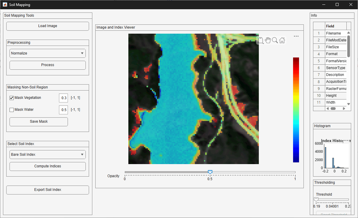
After computing the index, the function overlays the result on the original image using a jet colormap. An opacity slider, controlled by the adjustOpacity helper function, provides visual controls for interpreting the index map. The helper function is attached to the example as a supporting file.

function adjustOpacity(fig)
    slider = findobj(fig, 'Tag', 'opacitySlider');
    opacity = slider.Value;

    if  isvalid(fig.UserData.Viewer.CurrentObject)
        fig.UserData.Viewer.CurrentObject.OverlayAlpha = opacity;
    end
end

Apply Thresholding to the Index Map

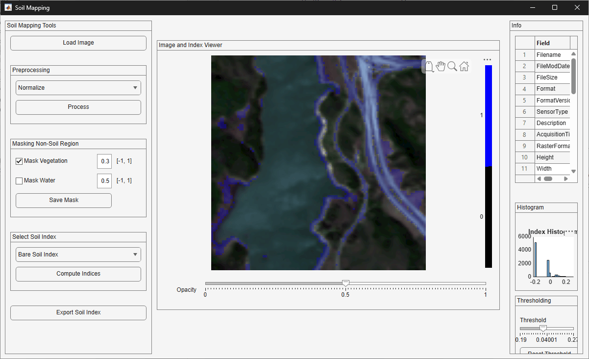
After computing a soil index, you can apply a threshold to classify pixels into two categories: above or below the threshold value. This produces a binary map useful for identifying regions with specific soil characteristics, such as areas with high clay content or elevated organic matter.

The right panel contains a threshold slider whose limits update dynamically based on the computed index range. As you adjust the slider, the applyThreshold helper function generates a binary overlay and updates the colorbar to reflect the two-class display. The helper function is attached to the example as a supporting file.

function applyThreshold(fig)
    if ~isfield(fig.UserData, "IndexMap")
        return;
    end

    idxMap = fig.UserData.IndexMap;
    threshold = findobj(fig, 'Tag', 'thresholdSlider').Value;

    ax = fig.UserData.Viewer;

    % Apply threshold to create binary mask
    binaryMask = idxMap > threshold;

    % Display thresholded mask
    ax.CurrentObject.OverlayData = binaryMask;

    % update colorbar
    updateBinaryColorbar(fig);

    % Enable reset button
    btnReset = findobj(fig, 'Tag', 'resetThresholdButton');
    if ~isempty(btnReset)
        btnReset.Enable = 'on';
    end
end

To return to the continuous index view, select the Reset Threshold button. This restores the original colormap and resets the slider to the minimum index value using the resetThreshold helper function. The helper function is attached to the example as a supporting file.

function resetThreshold(fig)
    % reset Threshold
    idxMap = fig.UserData.IndexMap;
    % Display (overlay index map)
    ax = fig.UserData.Viewer;
    ax.CurrentObject.OverlayData = rescale(idxMap,0,255);
    ax.CurrentObject.OverlayColormap = jet(256);

    % Update slider limits and make threshold panel visible
    sld = findobj(fig, 'Tag', 'thresholdSlider');

    minVal = double(min(idxMap(:), [], 'omitnan'));
    maxVal = double(max(idxMap(:), [], 'omitnan'));
    sld.Limits = [minVal, maxVal];
    sld.Value = minVal;

    % Restore continuous colorbar
    updateColorbar(fig, maxVal, minVal);

    % Disable Reset button
    btnReset = findobj(fig, 'Tag', 'resetThresholdButton');
    if ~isempty(btnReset)
        btnReset.Enable = 'off';
    end
end

Export the Soil Index Map

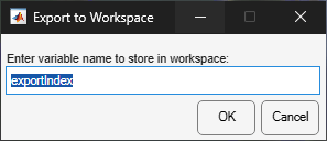
The exportMap helper function saves the computed soil index to the MATLAB base workspace. When you select Export Soil Index, a dialog prompts you to specify a variable name. The function validates the name and assigns the index map to the workspace for further processing or file export. The helper function is attached to the example as a supporting file.

function exportMap(fig)
    if ~isfield(fig.UserData, "IndexMap")
        uialert(fig, "No index has been computed yet.", "Export Failed");
        return;
    end
    
    img = fig.UserData.IndexMap;

    % Ask user for variable name
    defaultName = "exportIndex";
    prompt = {'Enter variable name to store in workspace:'};
    dlgTitle = 'Export to Workspace';
    dims = [1 50];
    answer = inputdlg(prompt, dlgTitle, dims, {defaultName});
    
    if isempty(answer), return; end  % User cancelled
    varName = matlab.lang.makeValidName(answer{1});

    % Assign to base workspace
    assignin('base', varName, img);

    uialert(fig, "Exported as '" + varName + "' to base workspace.", "Export Successful","Icon","success");
end

Run the Soil Mapping App

To use the app, load a hypercube or multicube object into the MATLAB workspace.

hcube = imhypercube("jasperRidge2_R198.img");

Then run the soilMappingApp function.

soilMappingApp

After the app opens, follow this workflow.

1. Select Load Image and select a hyperspectral data variable from the workspace.

2. Optionally, select a preprocessing method and select Process to prepare the data.

3. Optionally, enable vegetation or water masking and select Save Mask to exclude non-soil regions.

4. Select a soil index from the dropdown and select Compute Indices to generate the index map. The result overlays on the image in the viewer.

5. Use the opacity slider to adjust the overlay transparency and the threshold slider to classify the index values.

6. Select Export Soil Index to save the computed map to the workspace.