Augment Known Linear Model with Flexible Nonlinear Functions

This example demonstrates a method to improve the normalized root mean-squared error (NRMSE) fit score of an existing state-space model using a neural state-space model.

The structure of a discrete-time state-space model is:

$x_{k+1}=A{x}_k+B{u}_k$

$$y_k=x_k$$

Here, $$A{x}_k+B{u}_k$$ represents the known linear part of the dynamics. You can compute $$A$$ and $$B$$ matrices from prior knowledge (for example, from physical modeling), or from prior linear estimation. In this example, you extend the state transition dynamics by adding a nonlinear function, $$f(x_k,u_k)$$, represented by a neural network. To do this, you use a neural state-space model that uses a custom neural network.

The structure of the discrete-time neural state-space model is:

$x_{k+1}=A{x}_k+B{u}_k+f(x_k,u_k)$

$$y_k=x_k$$

Model Description

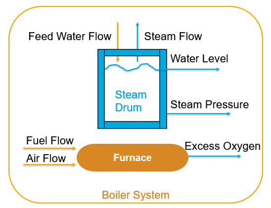
This example considers the dynamics of a steam generator at the Abbott Power Plant in Champaign, IL. While a linear model provides a good baseline model, it is not enough for capturing the smaller nonlinear contributions to the dynamics. So you use a model which is a nonlinear system with four inputs and four outputs. It faithfully displays all the essential features of the actual boiler dynamics including nonlinearities, nonminimum phase behaviors, instabilities, noise spectrum, time delays, and load disturbances. For more information on the model, see [1].

Data Preparation

Load the data set. Prepare both the estimation and validation data.

load boiler.mat z
z.OutputName = {'Drum Pressure', 'Excess Oxygen Level', ...
   'Drum Water Level','Steam Flow Rate'};
z.InputName = {'Fuel Flow Rate', 'Air Flow Rate', ...
   'Feed Water Flow Rate','Load Disturbance'};
ze = z(1:7000);
ze.Name = "estimation data";
zv = z(7001:end); 
zv.Name = "validation data";

Display the data set.

stackedplot(iddata2timetable(ze),iddata2timetable(zv))

To ensure that all features have the same scale, normalize the data set. This helps avoid numerical errors during training.

ze.y = normalize(ze.y);
ze.u = normalize(ze.u);
zv.y = normalize(zv.y);
zv.u = normalize(zv.u);

Linear Model Estimation

To estimate the linear model, you can use:

1. Empirical or physical laws incorporating simplifying assumptions

2. A digital system in Simulink® and linearize it about a nominal operating condition

3. The ssest function

In this example, you set training options using ssestOptions and train a fourth-order linear state-space model using the ssest function.

nx = 4;
opt = ssestOptions;
opt.Focus = "simulation";
opt.OutputWeight = eye(nx);
opt.EstimateCovariance = false;
opt.SearchMethod = "lm";

rng("default");
sysd = ssest(ze,nx,opt,DisturbanceModel="none",Ts=3);

Transform the model so that it has y=x as its output equation. This is required to create a neural state-space model later.

linsys = ss2ss(sysd,sysd.C)

linsys =
  Discrete-time identified state-space model:
    x(t+Ts) = A x(t) + B u(t) + K e(t)
       y(t) = C x(t) + D u(t) + e(t)
 
  A = 
              x1         x2         x3         x4
   x1     0.9963    0.02005  -0.003057   -0.05075
   x2    0.02933     0.7955  -0.005347    0.02414
   x3    0.03075    -0.0462     0.9575    -0.1081
   x4    0.05099   -0.02074   0.007758     0.8997
 
  B = 
       Fuel Flow Ra  Air Flow Rat  Feed Water F  Load Disturb
   x1       0.06703     -0.009903      0.004164       0.01035
   x2       -0.1894        0.1014      -0.02146      0.008553
   x3       0.03703       0.02013       0.03299       0.06205
   x4       0.04863       0.01055      -0.01498       0.06012
 
  C = 
                         x1          x2          x3          x4
   Drum Pressur           1   4.718e-16  -1.055e-15  -3.331e-16
   Excess Oxyge           0           1           0           0
   Drum Water L           0  -9.021e-17           1  -5.551e-17
   Steam Flow R           0           0           0           1
 
  D = 
                 Fuel Flow Ra  Air Flow Rat  Feed Water F  Load Disturb
   Drum Pressur             0             0             0             0
   Excess Oxyge             0             0             0             0
   Drum Water L             0             0             0             0
   Steam Flow R             0             0             0             0
 
  K = 
       Drum Pressur  Excess Oxyge  Drum Water L  Steam Flow R
   x1             0             0             0             0
   x2             0             0             0             0
   x3             0             0             0             0
   x4             0             0             0             0
 
Sample time: 3 seconds

Parameterization:
   FREE form (all coefficients in A, B, C free).
   Feedthrough: yes
   Disturbance component: estimate
   Number of free coefficients: 80
   Use "idssdata", "getpvec", "getcov" for parameters and their uncertainties.

Status:                         
Model modified after estimation.
 

Compare the simulated model response with the validation data.

compare(zv,linsys)
legend('show',Location='bestoutside')

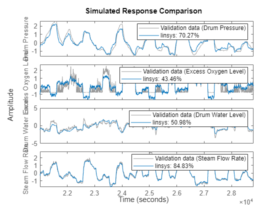
You can see that the linear model is not sufficient for estimation as the fit percentages for the second and third outputs are poor.

Nonlinear Model Estimation

First, create the state network used for training based on the state equation $x_{k+1}=A{x}_k+B{u}_k+f(x_k,u_k)$. The model has four states, four inputs, and a hidden layer of size 10.

nx = 4;
nu = 4;
nh = 10; 

Create a custom neural network to represent the state equation using the helper function createSSNN defined at the end of the example.

net = createSSNN(nx,nu,nh);  % x(k+1) = Ax + Bu + f(x,u)

Initialize the weights and biases corresponding to A and B based on their values from the linear model.

A = linsys.A;
B = linsys.B;
ind = 7;
net.Learnables{ind,3} = {dlarray(A)};  % weight for A
net.Learnables{ind+1,3} = {dlarray(zeros(nx,1))}; % bias for A
net.Learnables{ind+2,3} = {dlarray(B)}; % weight for B
net.Learnables{ind+3,3} = {dlarray(zeros(nx,1))}; % bias for B
plot(net)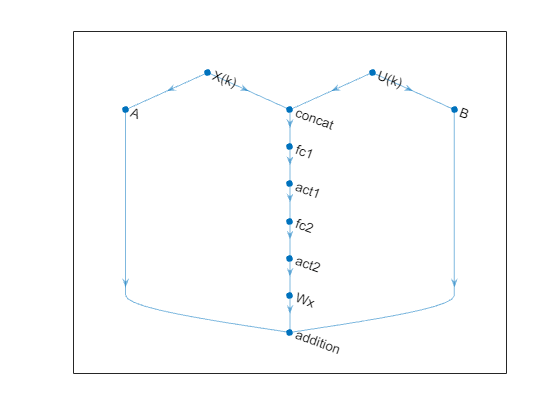

Use idNeuralStateSpace to create the neural state-space model using the same sample time as the linear model. Assign the created custom network as the state network of the model.

nss = idNeuralStateSpace(nx,NumInputs=nu,Ts=linsys.Ts);
nss.StateNetwork = net;

Warning: By default, "X(k)" layer is used as state and "U(k)" layer is used as input. If this is not the case, consider using "setNetwork" to assign the layer names.

To avoid the warning, you can use the setNetwork function.

nss = setNetwork(nss,"state",net,xName='X(k)',uName='U(k)');

Set the training options using nssTrainingOptions. To avoid simulating over the entire data set, split the data set into small segments using the WindowSize and Overlap properties. This speeds up training and improves model performance. To enable mini-batch learning, set NumWindowFraction to 0.3. In each iteration, the software randomly selects 30% of the data and updates the network parameters.

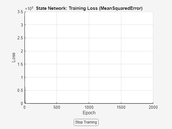
Train the model using nlssest.

opts = nssTrainingOptions('adam');
opts.MaxEpochs = 2000;
opts.LearnRate = 0.1;
opts.WindowSize = 150;
opts.Overlap = 30;
opts.NumWindowFraction = 0.3;
opts.LossFcn = "MeanSquaredError";
opts.LearnRateSchedule = "piecewise";
opts.LearnRateDropFactor = 0.5;
opts.LearnRateDropPeriod = 300;

UseTrainedModel = true;
if UseTrainedModel
    load modelA.mat sys
    sys
else
    sys = nlssest(ze,nss,opts) %#ok<UNRCH>
end

sys =

Discrete-time Neural ODE in 4 variables
     x(t+1) = f(x(t),u(t))
       y(t) = x(t) + e(t)
 
f(.) network:
  Deep network with 4 fully connected, hidden layers
  Activation function: sigmoid
 
Variables: x1, x2, x3, x4
Sample time: 3 seconds
 
Status:                                          
Estimated using NLSSEST on time domain data "ze".
Fit to estimation data: [87.7;78.77;74.44;88.08]%
FPE: 6.391e-07, MSE: 0.1397

Compare the simulated linear and nonlinear model responses with the validation data.

compare(zv,linsys,sys)
legend('show',Location='bestoutside')

Verify that the weights corresponding to A and B are same as those of the linear model.

A_trained = extractdata(sys.StateNetwork.Learnables.Value{7});
norm(A-A_trained,inf)

ans = 
2.8892e-12

B_trained = extractdata(sys.StateNetwork.Learnables.Value{9});
norm(B-B_trained,inf)

ans = 
1.9660e-12

You can observe that the neural state-space model successfully captures the unmodeled dynamics with the linear part fixed.

Function to Create Neural Network

Create a custom neural network representing $$x(k+1)=Ax+Bu+f(x,u)$$.

function net = createSSNN(nx,nu,nh)
net = dlnetwork;

% Input layers for x and u
tempLayers = featureInputLayer(nx,"Name","X(k)");
net = addLayers(net,tempLayers);
tempLayers = featureInputLayer(nu,"Name","U(k)");
net = addLayers(net,tempLayers);

% Layers for f(x,u)
tempLayers = [
    concatenationLayer(1,2,"Name","concat") 
    fullyConnectedLayer(nh,"Name","fc1")
    sigmoidLayer("Name","act1")
    fullyConnectedLayer(nh,"Name","fc2")
    sigmoidLayer("Name","act2")
    fullyConnectedLayer(nx,"Name","Wx")];
net = addLayers(net,tempLayers);

% Layers for Ax
tempLayers = fullyConnectedLayer(nx,"Name","A");
tempLayers.WeightLearnRateFactor = 0; % Fix linear component of model
tempLayers.BiasLearnRateFactor = 0;
net = addLayers(net,tempLayers);

% Layers for Bu
tempLayers = fullyConnectedLayer(nx,"Name","B");
tempLayers.WeightLearnRateFactor = 0; % Fix linear component of model
tempLayers.BiasLearnRateFactor = 0;
net = addLayers(net,tempLayers);

% Layers for f(x,u)
tempLayers = additionLayer(3,"Name","addition");
net = addLayers(net,tempLayers);

% Connect all branches of the network to create the network graph
net = connectLayers(net,"X(k)","concat/in1");
net = connectLayers(net,"X(k)","A");
net = connectLayers(net,"U(k)","concat/in2");
net = connectLayers(net,"U(k)","B");
net = connectLayers(net,"A","addition/in1");
net = connectLayers(net,"B","addition/in2");
net = connectLayers(net,"Wx","addition/in3");

% Initialize the network
net = initialize(net);
end

References

1] G. Pellegrinetti and J. Benstman, Nonlinear Control Oriented Boiler Modeling - A Benchmark Problem for Controller Design, IEEE Tran. Control Systems Tech. Vol.4 No.1 Jan.1996