Main Content

translatecov

Translate parameter covariance across model transformation operations

    Description

    newSys = translatecov(fcn,sys) transforms sys into sysNew = fcn(sys) and translates the parameter covariance of sys to the parameter covariance of the transformed model. fcn is a transformation function that you specify. The command computes the parameter covariance of sys using the Gauss Approximation formula. For more information, see Algorithms.

    Applying model transformations directly does not always translate the parameter covariance of the original model to that of the transformed model. For example, d2c(sys) does not translate the parameter covariance of sys. In contrast, translatecov(@(x)d2c(x),sys) produces a transformed model that has the same coefficients as d2c(sys) and has the translated parameter covariance of sys.

    example

    newSys = translatecov(fcn,Input1,...,InputN) returns the model sys_new = fcn(Input1,...,InputN) and its parameter covariance. At least one of the N inputs must be a linear model with parameter covariance information.

    example

    Examples

    collapse all

    Convert an estimated transfer function model into state-space model while also translating the estimated parameter covariance.

    Estimate a transfer function model.

    load iddata1
    sys1 = tfest(z1,2);

    Convert the estimated model to state-space form while also translating the estimated parameter covariance.

    sys2 = translatecov(@(x)idss(x),sys1);

    If you convert the transfer function model to state-space form directly, the estimated parameter covariance is lost (the output of getcov is empty).

    sys3 = idss(sys1);
    getcov(sys3)
    ans =
    
         []
    

    View the parameter covariance in the estimated and converted models.

    covsys1 = getcov(sys1);
    covsys2 = getcov(sys2);

    Compare the confidence regions.

    h = bodeplot(sys1,sys2);
    showConfidence(h,2);

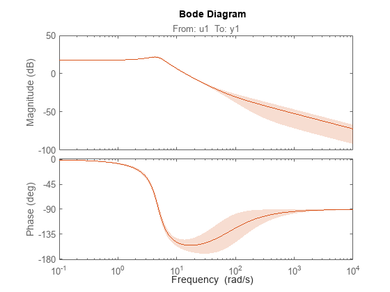
    MATLAB figure

    The confidence bounds for sys1 overlaps with sys2.

    Concatenate 3 single-output models such that the covariance data from the 3 models combine to produce the covariance data for the resulting model.

    Construct a state-space model.

    a = [-1.1008 0.3733;0.3733 -0.9561];
    b = [0.7254 0.7147;-0.0631 -0.2050];
    c = [-0.1241 0; 1.4897 0.6715; 1.4090 -1.2075];
    d = [0 1.0347; 1.6302 0; 0.4889 0];
    sys = idss(a,b,c,d,'Ts',0);

    Generate multi-output estimation data.

    t = (0:0.01:0.99)';
    u = randn(100,2);
    y = lsim(sys,u,t,'zoh');
    y = y +  rand(size(y))/10;
    data = iddata(y,u,0.01); 

    Estimate a separate model for each output signal.

    m1 = ssest(data(:,1,:),2,'feedthrough',true(1,2), 'DisturbanceModel', 'none');
    m2 = ssest(data(:,2,:),2,'feedthrough',true(1,2), 'DisturbanceModel', 'none');
    m3 = ssest(data(:,3,:),2,'feedthrough',true(1,2), 'DisturbanceModel', 'none');

    Combine the estimated models while also translating the covariance information.

    f = @(x,y,z)[x;y;z];
    M2 = translatecov(f, m1, m2, m3);

    The parameter covariance is not empty.

    getcov(M2, 'factors')
    ans = struct with fields:
           R: [36x36 double]
           T: [24x36 double]
        Free: [90x1 logical]


    If you combine the estimated models into one 3-output model directly, the covariance information is lost (the output of getcov is empty).

    M1 = [m1;m2;m3];
    getcov(M1)
    ans =
    
         []
    

    Compare the confidence bounds.

    h = bodeplot(M2, m1, m2, m3);
    showConfidence(h);

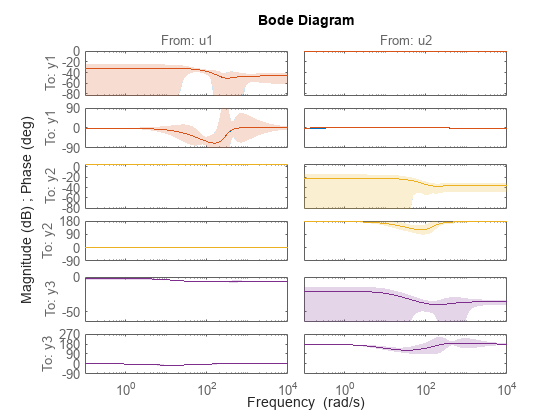
    MATLAB figure

    The confidence bounds for M2 overlap with those of m1, m2 and m3 models on their respective plot axes.

    Consider a closed-loop feedback model consisting of a plant and controller. Translate the parameter covariance of the plant to the closed-loop feedback model.

    Estimate a plant as a fourth-order state-space model using estimation data z1.

    load iddata1 z1
    Plant = ssest(z1,4);

    Plant contains parameter covariance information.

    Create a controller as a continuous-time zero-pole-gain model with zeros, poles, and gain equal to -2, -10, 5, respectively.

    Controller = zpk(-2,-10,5);

    Define a transformation function to generate the closed-loop feedback state-space model.

    fcn = @(x,y)idss(feedback(x,y));

    Translate the parameter covariance of the plant to the closed-loop feedback model.

    sys_new = translatecov(fcn,Plant,Controller);

    sys_new contains the translated parameter covariance information.

    Plot the frequency-response of the transformed model sys_new, and view the confidence region of the response.

    h = bodeplot(sys_new);
    showConfidence(h);

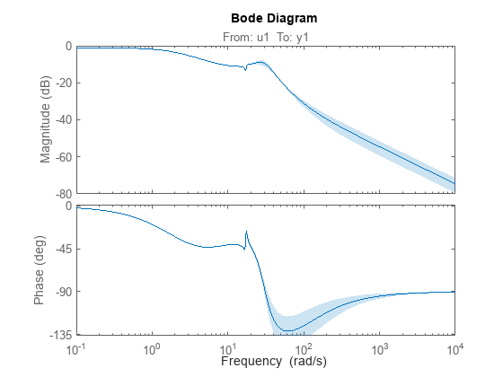
    MATLAB figure

    The plot shows the effect of the uncertainty in Plant on the closed-loop response.

    Input Arguments

    collapse all

    Model transformation function, specified as a function handle with one of the following syntaxes.

    • Single input — sysNew = fcn(sys)

    • Multiple inputs — sysNew = fcn(Input1,..InputN)

    If fcn has one input argument, the input must be a linear identified model with parameter covariance information. Typical single-input transformation operations include:

    • Convert to different model type, such as idpoly and idss. For example, fcn = @(x)idpoly(x) converts the model x to a polynomial model.

    • Change model sample time using, for example, c2d or d2c. For example, fcn = @(x)c2d(x,Ts) converts the continuous-time model x to a discrete-time model with sample time Ts.

    If fcn has multiple input arguments, at least one input argument must be an identified model with parameter covariance information (see sys). Typical multi-input operations include merging and concatenating of multiple models. For example, fcn = @(x,y)[x,y] performs horizontal concatenation of the models x and y.

    Linear identified model to use as input for transformation function fcn, returned as one of the following identified model objects.

    Multiple input arguments to the translation function fcn. At least one of the inputs must be a linear identified model with parameter covariance information. The other inputs can be any MATLAB data type.

    Output Arguments

    collapse all

    Model resulting from transformation, which includes parameter covariance information, returned as an identified model object.

    To view the translated parameter covariance, use getcov.

    Tips

    • If you obtained sys through estimation and have access to the estimation data, you can use zero-iteration update to recompute the parameter covariance. For example:

      load iddata1
      m = ssest(z1,4);
      opt = ssestOptions
      opt.SearchOptions.MaxIterations = 0;
      m_new = ssest(z1,m2,opt)
      

      You cannot run a zero-iteration update for some model and data type combinations, such as a continuous-time idpoly model using time-domain data.

      Also, you cannot run a zero-iteration update if the MaxIterations option, which depends on the SearchMethod option, is not available.

    Algorithms

    translatecov uses numerical perturbations of individual parameters of sys to compute the Jacobian of fcn(sys) parameters with respect to parameters of sys. translatecov then applies Gauss Approximation formula cov_new=J×cov× JT to translate the covariance, where J is the Jacobian matrix. This operation can be slow for models containing a large number of free parameters.

    Version History

    Introduced in R2012b