Main Content

Estimate Process Model

Estimate continuous-time process model for single-input, single-output (SISO) system in either time or frequency domain in the Live Editor

Description

The Estimate Process Model task lets you interactively estimate and validate a process model for SISO systems. You can define and vary the model structure and specify optional parameters, such as initial condition handling and search methods. The task automatically generates MATLAB® code for your live script. For more information about Live Editor tasks generally, see Add Interactive Tasks to a Live Script.

Process models are simple continuous-time transfer functions that describe the linear system dynamics. Process model elements include static gain, time constants, time delays, integrator, and process zero.

Process models are popular for describing system dynamics in numerous industries and are applicable to various production environments. The advantages of these models are that they are simple, they support transport delay estimation, and the model coefficients are easy to interpret as poles and zeros. For more information about process model estimation, see What Is a Process Model?

The Estimate Process Model task is independent of the more general System Identification app. Use the System Identification app when you want to compute and compare estimates for multiple model structures.

To get started, load experiment data that contains input and output data into your MATLAB workspace and then import that data into the task. Then select a model structure to estimate. The task gives you controls and plots that help you experiment with different model structures and compare how well the output of each model fits the measurements.

Related Functions

The code that Estimate Process Model generates uses the following functions.

The task estimates an idproc process model.

Estimate Process Model task in Live Editor

Open the Task

To add the Estimate Process Model task to a live script in the MATLAB Editor:

  • On the Live Editor tab, select Task > Estimate Process Model.

  • In a code block in your script, type a relevant keyword, such as process or estimate. Select Estimate Process Model from the suggested command completions.
Examples

expand all

Use the Estimate Process Model Live Editor Task to estimate a process model and compare the model output to the measurement data.

Set Up Data

Load the measurement data tt1 into your MATLAB workspace. tt1 is a timetable that contains one input variable u and one output variable y.

load sdata1 tt1

Import Data into the Task

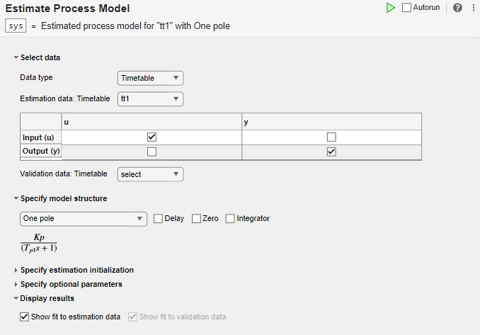
In the Select data section, set Data Type to Timetable and set Estimation Object to tt.

The task displays a table that contains the tt1 input and output variable names.

Estimate the Model Using Default Settings

Examine the model structure and optional parameters.

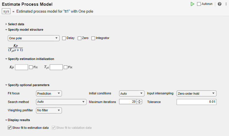
In the Specify model structure section, the default option is One Pole with no delay, zero, or integrator. Equations below the parameters in this section display the specified structure.

In the Specify estimation initialization section, initialization parameters matching the parameters in your model structure allow you to set starting points for estimation. If you select Fix, the parameter remains fixed to the value you specify. For this example, do not specify initialization. The task then uses default values for starting points.

In the Specify optional parameters section, the default options for process estimation are set.

Execute the task from the Live Editor tab by clicking the green arrow. You can also select Autorun to run the task automatically every time you update a parameter.

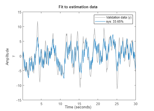
A plot displays the estimation data, the estimated model output, and the fit percentage.

Experiment with Parameter Settings

Experiment with the parameter settings and see how they influence the fit.

For instance, add delay to the One Pole structure and run the task.

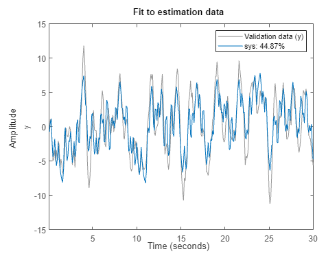
The estimation fit improves, although the fit percentage is still below 50%.

Try a different model structure. In Specify model structure, select Underdamped Pair with no delay and run the task.

The fit results improve significantly.

Generate Code

To display the code that the task generates, click at the bottom of the parameter section. The code that you see reflects the current parameter configuration of the task.

Use separate estimation and validation data so that you can validate the estimated process model.

Set Up Data

Load the measurement data iddata1 into your MATLAB workspace and examine its contents.

load sdata1 umat1 ymat1 Ts

Split the data into two sets, with one half for estimation and one half for validation. The original data set has 300 samples, so each new data set has 150 samples.

u_est = umat1(1:150);
u_val = umat1(151:300);
y_est = ymat1(1:150);
y_val = ymat1(151:300);
Ts
Ts = 
0.1000

Import Data into Task

In the Select data section, set Data Type to Numeric. Set the sample time to 0.1 seconds, which is 0.1 seconds. Select the appropriate data sets for estimation and validation.

Estimate and Validate the Model

The example Estimate Process Model with Live Editor Task achieves the best results using the model structure Underdamped Pair. Choose the same option for this example.

Execute the task. Executing the task creates two plots. The first plot shows the estimation results and the second plot shows the validation results.

The fit to the estimation data is somewhat worse than in Estimate Process Model with Live Editor Task. Estimation in the current example has only half the data with which to estimate the model. The fit to the validation data, which represents the goodness of the model more generally, is better than the fit to the estimation data.

Parameters

expand all

Select Data

The task accepts numeric measurement values that are uniformly sampled in time. Input and output signals can contain multiple channels. Data can be packaged as numeric arrays (for Numeric or Frequency), as a timetable, or in a data object, such as an iddata or idfrd object. For multiexperiment data, numeric and timetable data can be packaged as cell arrays. For cell arrays of timetables, all timetables must contain the same variable names. Data objects handle multiexperiment data internally.

The data type you choose determines whether you must specify additional parameters.

  • Numeric — Specify Sample Time and Start Time in the time units that you select.

  • Timetable — Specify no additional parameters because the timetable already contains information on sample time and start time.

  • Frequency — Specify Frequency by selecting the variable name of a frequency vector in your MATLAB workspace. Specify the units for this frequency vector. Specify Sample Time in seconds.

  • Data Object — Specify no additional parameters because the data object already contains information on time or frequency sampling.

Select the input and output variable names from the MATLAB workspace choices. Use these parameters when Data Type is Numeric or Frequency.

Specifying validation data is optional but recommended.

Select the timetable variable name from the MATLAB workspace choices. Use this parameter when Data Type is Timetable. The task displays the timetable variable names for the input and output. Estimation and validation timetables must contain the same variable names.

Select the data object variable name from the MATLAB workspace choices. Use this parameter when Data Type is Data Object.

Specify Model Structure

The task allows you to specify one of four basic structures. These structures range from a simple first-order process to a more dynamic second-order or third-order process with complex conjugate (underdamped) poles.

  • One Pole

  • Two Real Poles

  • Underdamped Pair

  • Underdamped Pair + Real Pole

Include transport delay, or input-to-output delay, of one sample. The transport delay is also known as dead time.

Include a process zero in the numerator.

Include an integrator, represented by an additional 1/ s term. Including an integrator creates a self-regulating process.

Specify Estimation Initialization

Specify initial values for the estimation and whether these values are to be fixed or estimated. The values to specify depend on the model structure and your specifications for Delay and Zero. Below Specify model structure, the task displays the equation that represents the specified system. This equation contains all of the parameters that can be estimated, and that you can initialize or fix. The possible parameters are:

  • Kp — Static gain

  • Tp1 — Time constant for first real pole

  • Tp2 — Time constant for second real pole

  • — Time constant for complex poles, equal to the inverse of the natural frequency

  • ζ — Damping coefficient for complex poles

  • Td — Transport delay

  • Tz — Time constant for the process zero

All time-based parameters are in the time units you select for Sample Time.

Specify Optional Parameters

Fit focus specifies what error to minimize in the loss function during estimation.

  • Prediction — Minimize the one-step-ahead prediction error between measured and predicted outputs. This estimation approach focuses on producing a good predictor model for the estimation inputs and outputs. Prediction focus generally produces the best estimation results because it uses both input and output measurements, thus accounting for disturbances.

  • Simulation — Minimize the error between measured and simulation outputs. This estimation approach focuses on producing a simulated model response that has a good fit with the estimation inputs and outputs. Simulation focus is generally best for validation, especially with data sets not used for the original estimation.

Set this option when you want to choose a specific method for initializing the model. With the default setting of Auto, the software chooses the method based on the estimation data. Choices are:

  • Zero — The initial state is set to zero.

  • Estimate — The initial state is treated as an independent estimation parameter.

  • Backcast — The initial state is estimated using the best least squares fit.

Input intersampling is a property of the input data. The task uses this property when estimating process models. Specify Input Intersampling when your data type is Time or Frequency. If you are using an iddata object, the object already contains the intersampling information. Choices for this property are:

  • Zero-order hold — Piecewise-constant input signal between samples

  • Triangle approximation — Piecewise-linear input signal between samples, also known as first-order hold

  • Band-limited — Input signal has zero power above the Nyquist frequency

  • Auto — For each iteration, the software cycles through the methods until it finds the first direction descent that leads to a reduction in estimation cost.

  • Gauss-Newton — Subspace Gauss-Newton least-squares search.

  • Levenberg-Marquardt — Levenberg-Marquardt least-squares search.

  • Adaptive Gauss-Newton —Adaptive subspace Gauss-Newton search.

  • Gradient Search — Steepest descent least-squares search.

Set the maximum number of iterations during error minimization. The iterations stop when Max. Iterations is reached or another stopping criterion is satisfied, such as Tolerance.

When the percentage of expected improvement is less than Tolerance, the iterations stop.

Set this option when you want to apply a weighting prefilter to the loss function that the task minimizes when you estimate the model. When you select an option, you must also select the associated variable in your workspace that contains the filter information. The available options depend on the domain of the data.

Weighting PrefilterData DomainFilter Information
No FilterTime and frequency 
PassbandsTime and frequencyPassband ranges, specified as a 1-by-2 row vector or an n-by-2 matrix, where n is the number of passbands
LTI FilterTime and frequencySISO LTI model
Frequency Weights VectorFrequencyFrequency weights, specified as a column vector with the same length as the frequency vector

For instance, suppose that you are performing estimation with SISO frequency-domain data and that in your MATLAB workspace, you have a column vector W that contains frequency weights for the prefilter. In the task, select Weighting prefilter > Frequency weights vector and the variable W.

Visualize Results

Plot a comparison of the model output and the original measured data, along with the fit percentage. If you have separate validation data, a second plot compares the model response to the validation input data with the measured output from the validation data set.

Version History

Introduced in R2019b

expand all

See Also

| | | | | | | (Control System Toolbox)

Go to top of page