Initialize a System-Level Heat Exchanger

This example shows how to specify the initial conditions for a system-level heat exchanger to prevent transient behavior at the start of the simulation. Properly specifying initial conditions can prevent unwanted behavior at the start of the simulation, such as spikes in values.

Your initialization solution depends on your model requirements:

• Start model near steady-state - Select the Initialize fluid to nominal operating conditions parameter for both fluids in the heat exchanger.

• Start model from rest - Specify a scalar value for the initial conditions on both sides of the heat exchanger to provide a uniform resting fluid state. Start flow sources, pumps, and compressors at rest. As the pumps and compressor gradually ramp up, the heat transfer will correspondingly ramp up.

• Start not at steady-state and not at rest - Specify the initial conditions as a two-element vector.

Examine Model with Constant Initial Conditions

For an example of transient behavior at the start of the simulation, open and run the InitializeASystemLevelHeatExchanger model, which contains a System-Level Condenser Evaporator (2P-TL) block. The initial temperature of the two-phase fluid side of the heat exchanger is 380 K, and the initial temperature of the thermal liquid size is 328 K.The temperature of the fluid in the reservoirs that feed the heat exchanger is the same as the initial conditions of the fluids in the heat exchanger.

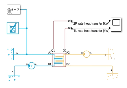
Simulate the model.

mdl = "InitializeASystemLevelHeatExchanger";
open_system(mdl);
sim(mdl);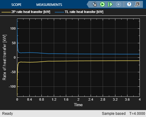

Because the initial conditions are specified as scalar, the block assumes that the scalar describes uniform conditions along the entire flow path. When the simulation starts, there is a 52 K temperature difference across the length of the heat exchanger flow path, which causes a large initial value for the heat transfer rate. The heat transfer rate quickly falls to the steady-state value, which is lower because the temperature of the two fluids approach each other as they travel inside the heat exchanger. By the time the fluids exit the heat exchanger, the temperature difference is less than 52 K. The large initial value and fast drop to steady-state conditions appear as initial transients in the heat transfer rate.

Start Model Near Steady-State Conditions

To start a model near steady-state conditions, reduce initial transients by initializing to nominal operating conditions. Use this approach when the boundary conditions in the model match the nominal operating conditions of the block. If the boundary conditions do not match the block nominal operating conditions, then the initialization matches the nominal conditions and not the steady-state conditions.

To initialize to nominal operating conditions, in the System-Level Condenser Evaporator (2P-TL) block, select Initialize two-phase fluid to nominal operating conditions and Initialize thermal liquid to nominal operating conditions. When you select these parameters, the block determines the distribution of temperatures between ports A and B based on the nominal operating condition parameters and the fluid states at the ports. Simulate the model.

set_param(mdl + "/System-Level Condenser Evaporator (2P-TL)", "nominal_init_2P", "true")
set_param(mdl + "/System-Level Condenser Evaporator (2P-TL)", "nominal_init_TL", "true")
sim(mdl);

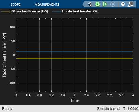
Because the steady state-conditions match the nominal operating conditions, there are no initial transients and the block initializes cleanly.

Revert these changes to reuse the model.

set_param(mdl + "/System-Level Condenser Evaporator (2P-TL)", "nominal_init_2P", "false")
set_param(mdl + "/System-Level Condenser Evaporator (2P-TL)", "nominal_init_TL", "false")

Start Model From Rest

To start a model from rest, start the model with no flow and then slowly increase it. Open the InitializeASystemLevelHeatExchangerRest model. This model is the same as the InitializeASystemLevelHeatExchanger model, except that it has two PS Transfer Function blocks that slow the flow rate and pressure differential on the Thermal Liquid and Two-Phase Fluid sides of the heat exchanger, respectively. The initial conditions on both sides of the heat exchanger are scalar temperatures.

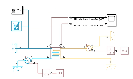
Simulate the model and plot the output from both PS Transfer Function blocks. These signals are the input to the Pressure Source (2P) and Flow Rate Source (TL) blocks in the model.

mdl_rest = "InitializeASystemLevelHeatExchangerRest";
open_system(mdl_rest);
sim(mdl_rest);
time = tout;
pressure_diff_2p = simlog_InitializeASystemLevelHeatExchangerRest.PS_Transfer_Function.Y.series.values("kPa"); 
flow_rate_TL = simlog_InitializeASystemLevelHeatExchangerRest.PS_Transfer_Function1.Y.series.values("kg/s");
Q1 =  simlog_InitializeASystemLevelHeatExchangerRest.System_Level_Condenser_Evaporator_2P_TL.Q1.series.values("kW"); 
Q2 =  simlog_InitializeASystemLevelHeatExchangerRest.System_Level_Condenser_Evaporator_2P_TL.Q2.series.values("kW"); 

figure;
yyaxis left;
plot(time, pressure_diff_2p, "DisplayName", "Pressure Differential (2P) [kPa]","LineWidth",2);
ylabel("Pressure Differential (2P) [kPa]");
grid on;

yyaxis right;
plot(time, flow_rate_TL,"--","DisplayName", "Flow Rate (TL) [kg/s]","LineWidth",2);
ylabel("Flow Rate (TL) [kg/s]");
xlabel("Time [s]");
title("Pressure Differential and Flow Rate over Time");
legend("show");

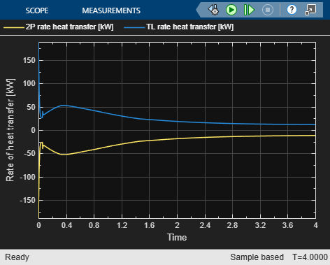
This figure shows that the input signals to the Pressure Source (2P) and Flow Rate Source (TL) blocks slowly increase over the simulation. Plot the rate of heat transfer on both sides of the heat exchanger.

figure
plot(time,Q1,time,Q2,"LineWidth",2)
ylabel("Rate of heat transfer [kW]");
xlabel("Time [s]");
legend("2P rate heat transfer [kW]","TL rate heat transfer [kW]")

Because the fluid flow slowly increases, the rate of heat transfer also slowly increases, which prevents initial transients, even though there is a large temperature difference across the heat exchanger at the start of the simulation.

Start Not at Steady-State and Not at Rest

To initialize the model neither at steady-state nor at rest, specify the initial conditions as a two-element vector. When you specify a two-element vector, the block assumes that the initial condition varies linearly between ports A and B, where the first element corresponds to port A and the second element corresponds to port B.

Open the InitializeASystemLevelHeatExchanger model. Assume that you want to initialize the model to 310 K on the thermal liquid side and 390 K on the two-phase fluid side. Specify the initial conditions and simulate the model with constant initial conditions.

set_param(mdl + "/System-Level Condenser Evaporator (2P-TL)", "T_init_TL", "310")
set_param(mdl + "/System-Level Condenser Evaporator (2P-TL)", "T_init_2P", "390")
sim(mdl);

Because the initial conditions are constant across the heat exchanger, and the model does not initialize at steady-state conditions, there is a spike in the rate of heat transfer at the start of the simulation. To help determine which temperatures to initialize to, plot the temperature of the thermal liquid and the two-phase fluid at the inlet and the outlet, and the two-phase fluid vapor quality at the inlet and outlet.

time = tout;
temp_TL_A = simlog_InitializeASystemLevelHeatExchanger.System_Level_Condenser_Evaporator_2P_TL.thermal_liquid_2.T_A.series.values("K");
temp_TL_B = simlog_InitializeASystemLevelHeatExchanger.System_Level_Condenser_Evaporator_2P_TL.thermal_liquid_2.T_B.series.values("K");
temp_2P_A = simlog_InitializeASystemLevelHeatExchanger.System_Level_Condenser_Evaporator_2P_TL.two_phase_fluid_1.T_A.series.values("K");
temp_2P_B = simlog_InitializeASystemLevelHeatExchanger.System_Level_Condenser_Evaporator_2P_TL.two_phase_fluid_1.T_B.series.values("K");
Q1_constant_IC = simlog_InitializeASystemLevelHeatExchanger.System_Level_Condenser_Evaporator_2P_TL.Q1.series.values("kW");
Q2_constant_IC = simlog_InitializeASystemLevelHeatExchanger.System_Level_Condenser_Evaporator_2P_TL.Q2.series.values("kW");
x_A = simlog_InitializeASystemLevelHeatExchanger.System_Level_Condenser_Evaporator_2P_TL.two_phase_fluid_1.x_A.series.values;
x_B = simlog_InitializeASystemLevelHeatExchanger.System_Level_Condenser_Evaporator_2P_TL.two_phase_fluid_1.x_B.series.values;
h_A = simlog_InitializeASystemLevelHeatExchanger.System_Level_Condenser_Evaporator_2P_TL.two_phase_fluid_1.h_A.series.values;
h_B = simlog_InitializeASystemLevelHeatExchanger.System_Level_Condenser_Evaporator_2P_TL.two_phase_fluid_1.h_B.series.values;
figure
plot(time,temp_TL_A,time,temp_TL_B,time,temp_2P_A,time,temp_2P_B,"LineWidth",2)
xlabel("Time [s]")
ylabel("Temperature [K]")
title("Temperature at TL and 2P Inlet and Outlet")
legend("TL inlet", "TL outlet","2P inlet", "2P outlet")

figure
plot(time,x_A,time,x_B,"LineWidth",2)
xlabel("Time [s]")
ylabel("Two-Phase Fluid Vapor Quality")
title("Fluid Vapor Quality at 2P Inlet and Outlet")
legend("2P inlet", "2P outlet")

To determine the two-element vector to use for the thermal liquid side, examine the inlet and outlet temperature plot. This plot shows that after the simulation starts, on the thermal liquid side, the temperature at the inlet and outlet both rise. Use this pattern to specify a two element vector initial conditions. On the thermal liquid side, set the outlet temperature higher than the input. Set the Initial thermal liquid temperature parameter to [310 350] K.

To determine the two-element vector to use for the two-phase fluid side, first examine the vapor quality plot. This plot shows that vapor quality drops below 1 at the two-phase outlet, which means that is becomes a saturated liquid-vapor mixture. To match this behavior, you cannot specify the two-phase fluid initial conditions at the outlet by using temperature, because a temperature value cannot uniquely determine the fluid state of a liquid-vapor mixture. Use specific enthalpy instead, which can uniquely define the fluid state. Plot the two-phase fluid specific enthalpy at the inlet and outlet.

figure
plot(time,h_A,time,h_B,"LineWidth",2)
xlabel("Time [s]")
ylabel("Two-Phase Fluid Specific Enthalpy [kJ/kg]")
title("Specific Enthalpy at 2P Inlet and Outlet")
legend("2P inlet", "2P outlet")

Use the specific enthalpy plot to choose initial conditions by choosing inlet and outlet enthalpy values that match the plot at the end of the simulation. Set Initial fluid energy specification to Specific enthalpy and Initial two-phase fluid specific enthalpy to [740 580] kJ/kg.

Specifying these values for the vector initial conditions does change the fluid state at the start of the simulation, because the temperature in the heat exchanger is 310 K and 390 K only at the thermal liquid and two-phase fluid entrances, respectively, rather than across the entire flow path. In your applications, use an iterative process to find the right balance between the desired initial state and avoiding transient behavior. The closer initial conditions are to steady-state, the smaller initial transients will be.

Simulate the model and plot the heat transfer over the first second for both the constant and linear initial conditions.

set_param(mdl + "/System-Level Condenser Evaporator (2P-TL)", "T_init_TL", "[310 340]")
set_param(mdl + "/System-Level Condenser Evaporator (2P-TL)", "energy_spec_2P","foundation.enum.energy_spec.enthalpy")
set_param(mdl + "/System-Level Condenser Evaporator (2P-TL)", "h_init_2P", "[740 580]")
set_param(mdl + "/Scope","open","off");
sim(mdl);
Q1_linear_IC = simlog_InitializeASystemLevelHeatExchanger.System_Level_Condenser_Evaporator_2P_TL.Q1.series.values("kW");
Q2_linear_IC = simlog_InitializeASystemLevelHeatExchanger.System_Level_Condenser_Evaporator_2P_TL.Q2.series.values("kW");
plot(time, Q1_constant_IC,time,Q2_constant_IC,tout,Q1_linear_IC,tout,Q2_linear_IC,"LineWidth",2)
xlabel("Time [s]")
ylabel("Rate of Heat Transfer [kW]")
title("Heat Transfer For Linear and Constant Initial Conditions")
xlim([0 1])
legend("2P Constant IC", "TL Constant IC","2P Linear IC", "TL Linear IC")

This plot shows that specifying the vector initial conditions reduces the spike in heat transfer rate at the beginning of the simulation. The heat transfer also reaches steady-state conditions faster and more smoothly.