Pipe (TL)
R2026bPipe that transports fluid in thermal liquid networks
Pipe (TL) block
To add a block to a model, double-click the canvas and start typing the block name. Then, select the block from the list.
Libraries:
Simscape /
Fluids /
Thermal Liquid /
Pipes & Fittings
Description
The Pipe (TL) block represents thermal liquid flow through a pipe. The block finds the temperature across the pipe from the differential between ports, pipe elevation, and any additional heat transfer at port H.
The pipe can have a constant or varying elevation between ports A
and B. For a constant elevation differential, use the
Elevation gain from port A to port B parameter. You can specify
a variable elevation by setting Elevation gain specification to
Variable. This exposes physical signal port
EL.
You can choose to include the effects of fluid dynamic compressibility, inertia, and wall flexibility. When the block includes these phenomena, it calculates the flow properties for each number of pipe segments that you specify.
Pipe Geometry
Use the Cross-sectional geometry parameter to specify the shape of the pipe.
The nominal hydraulic diameter, DN, and the pipe diameter, dcircle, are both equal to the is the value of the Pipe diameter parameter. The pipe cross-sectional area is
The nominal hydraulic diameter is the difference between the Pipe outer diameter and Pipe inner diameter parameters DN = douter – dinner. The pipe cross-sectional area is
The nominal hydraulic diameter is
where:
h is the is the value of the Pipe height parameter.
w is the is the value of the Pipe width parameter.
The pipe cross-sectional area is
The nominal hydraulic diameter is
where:
amaj is the is the value of the Pipe major axis parameter.
bmin is the is the value of the Pipe minor axis parameter.
The pipe cross-sectional area is
The nominal hydraulic diameter is
where:
lside is the is the value of the Pipe side length parameter.
θ is the is the value of the Pipe vertex angle parameter.
The pipe cross-sectional area is
When the Cross-sectional geometry parameter is
Custom, you can specify the pipe cross-sectional
area with the Cross-sectional area parameter. The nominal
hydraulic diameter is the value of the Hydraulic diameter
parameter.
Pipe Flexibility
You can model flexible walls for all cross-sectional geometries. When you set
Pipe wall specification to
Flexible, the block assumes uniform expansion along
all directions and preserves the defined cross-sectional shape. This setting may not
result in physical results for noncircular cross-sectional areas undergoing high
pressure relative to atmospheric pressure. When you model flexible walls, you can
use the Volumetric expansion specification parameter to specify
the volumetric expansion of the pipe cross-sectional area.
When the Volumetric expansion specification parameter is
Cross-sectional area vs. pressure, the change in
volume is
where:
L is the Pipe length parameter.
SN is the nominal pipe cross-sectional area defined for each shape.
S is the current pipe cross-sectional area.
p is the internal pipe pressure.
patm is either the atmospheric pressure or the value of the Environment pressure parameter, depending on the value of the Environment pressure specification parameter.
Kps is the Static gauge pressure to cross-sectional area gain parameter.
To calculate Kps assuming uniform elastic deformation of a thin-walled, open-ended cylindrical pipe, use
where t is the pipe wall thickness and E is Young's modulus.
τ is the Volumetric expansion time constant.
When the Volumetric expansion specification parameter is
Cross-sectional area vs. pressure - Tabulated, the
block uses the same equation for as the Cross-sectional area vs.
pressure setting. The block calculates A with
the table lookup function
where pps is the Static gauge pressure vector parameter and Aps is the Cross sectional area gain vector parameter.
When the Volumetric expansion specification parameter is
Hydraulic diameter vs. pressure, the change in volume is
where:
DN is the nominal hydraulic diameter defined for each shape.
D is the current pipe hydraulic diameter.
Kpd is the Static gauge pressure to hydraulic diameter gain parameter. To calculate Kps assuming uniform elastic deformation of a thin-walled, open-ended cylindrical pipe, use
When the Volumetric expansion specification parameter is
Based on material properties, the block uses the same
equation for as the Hydraulic diameter vs. pressure
setting but calculates Dstatic depending
on the value of the Material behavior parameter
This parameterization assumes a cylindrical thin-walled pressure vessel where
When the Material behavior parameter is Linear
elastic,
where:
E is the value of the Young's modulus parameter.
v is the value of the Poisson's ratio parameter.
, where t is the value of the Pipe wall thickness parameter.
When the Material behavior parameter is
Multilinear elastic, the block calculates the von
Mises stress, σv, which simplifies to , to determine the equivalent strain. The hoop strain is
where:
The block calculates the Young's Modulus, E, from the first elements of the Stress vector and Strain vector parameters.
, where σtotal and εtotal are the equivalent total stress and the equivalent total strain, respectively. The block calculates the equivalent total strain from the von Mises stress and the stress-strain curve.
where σi,j are the elements of the Cauchy stress tensor.
If you do not model flexible walls, SN = S and DN = D.
If you select Enable pipe thermal expansion, the block models the thermal expansion of the pipe wall using these assumptions:
The pipe material is isotropic.
The Biot number of the pipe is less than 0.1 and the pipe can be modeled with lumped thermal capacitance.
The temperature change and pipe deformations are small enough that a first order approximation for area expansion is accurate.
When the Material behavior parameter is
Cross-sectional area vs. pressure,
Cross-sectional
                        area vs. pressure - Tabulated
, or
Hydraulic diameter vs. pressure and you select
Enable pipe thermal expansion, the block adds a thermal
expansion term when calculating area or diameter.
When Material behavior is Cross-sectional
area vs. pressure,
where:
ɑ is the value of the Coefficient of thermal expansion parameter.
TI is the fluid temperature at the internal node of the block.
Tref is the value of the Thermal expansion reference temperature parameter.
When Material behavior is Cross-sectional
area vs. pressure - Tabulated,
When Material behavior is
Hydraulic diameter vs.
pressure,
When the Material behavior parameter is
Multilinear elastic and you select
Enable pipe thermal expansion, the block calculates
Dstatic as
where
Heat Transfer at the Pipe Wall
Heat transfer between the fluid and pipe wall occurs through convection, QConv and conduction, QCond, where the net heat flow rate, QH is QH=QConv+QCond.
Heat transfer due to conduction is:
where:
D is the nominal hydraulic diameter, DN, if the pipe walls are rigid, and is the pipe steady-state diameter, DS, if the pipe walls are flexible.
kI is the thermal conductivity of the thermal liquid, defined internally for each pipe segment.
SH is the surface area of the pipe wall.
TH is the pipe wall temperature.
TI is the fluid temperature at the internal node of the block.
Heat transfer due to convection is:
where:
cp, Avg is the average fluid specific heat which the block calculates using a lookup table.
Avg is the average mass flow rate through the pipe.
TIn is the fluid inlet port temperature.
h is the pipe heat transfer coefficient.
The heat transfer coefficient h is:
except when parameterizing by Nominal temperature
differential vs. nominal mass flow rate, where
kAvg is the average thermal
conductivity of the thermal liquid over the entire pipe and Nu is
the average Nusselt number in the pipe.
The block calculates the Nusselt number depending on the flow and the setting of Heat transfer parameterization. When Heat transfer parameterization is
Gnielinski correlationNominal temperature differential vs. nominal mass flow rateDittus-Boelter correlation - Nusselt = a * Re^b * Pr^c
and the flow is laminar, the block uses Nusselt number data and lookup tables to determine the Nusselt number. For the Nusselt number data that the block uses, see Algorithms. When the flow is turbulent, the block calculates the Nusselt number by using equations that depends on the correlation.
When Heat transfer parameterization is
Gnielinski correlation and the flow is turbulent,
the average Nusselt number is
where:
f is the average Darcy friction factor, according to the Haaland correlation,
where εR is the pipe value of the Internal surface absolute roughness parameter.
Re is the Reynolds number.
Pr is the Prandtl number.
When Heat transfer parameterization is
Dittus-Boelter correlation - Nusselt = a * Re^b *
                                    Pr^c
and the flow is turbulent, the average Nusselt number is
where:
a is the value of the Coefficient a parameter.
b is the value of the Exponent b parameter.
c is the value of the Exponent c parameter.
When Heat transfer parameterization is
Nominal temperature difference vs. nominal mass flow
rate and the flow is turbulent, the heat transfer coefficient is
where:
N is the value of the Nominal mass flow rate parameter.
Avg is the average mass flow rate,
hN is the nominal heat transfer coefficient,
where:
SH,N is the nominal wall surface area.
TH,N is the value of the Nominal wall temperature parameter.
TIn,N is the value of the Nominal inflow temperature parameter.
TOut,N is the value of the Nominal outflow temperature parameter.
This relationship assumes that the Nusselt number is proportional to the Reynolds number:
If the pipe walls are rigid, the expression for the heat transfer coefficient is
When the flow is turbulent, Cross-sectional geometry is
Annular, and Heat transfer
walls is Inner wall or
Outer wall, you can use the Nusselt
number correction factor parameter to specify a Nusselt number
correction term. When you set Nusselt number correction
factor to
When Heat transfer parameterizationis
Tabulated data - Colburn factor vs. Reynolds
number, the average Nusselt number is
where JM is the Colburn-Chilton factor.
When Heat transfer parameterization is
Tabulated data - Nusselt number vs. Reynolds number &
Prandtl number, the block interpolates the Nusselt number from
the three-dimensional array of average Nusselt numbers as a function of both the
average Reynolds number and average Prandtl number,
Pipe Effects
The block lets you include dynamic compressibility and fluid inertia effects. Turning on each of these effects can improve model fidelity at the cost of increased equation complexity and potentially increased simulation cost:
When you disable dynamic compressibility, the liquid is assumed to spend negligible time in the pipe volume. Therefore, there is no accumulation of mass in the pipe, and mass inflow equals mass outflow. This is the simplest option. It is appropriate when the liquid mass in the pipe is a negligible fraction of the total liquid mass in the system.
When you enable dynamic compressibility, an imbalance of mass inflow and mass outflow can cause liquid to accumulate or diminish in the pipe. As a result, pressure in the pipe volume can rise and fall dynamically, which provides some compliance to the system and modulates rapid pressure changes. This is the default option.
If dynamic compressibility is enabled, you can also turn on fluid inertia. This effect results in additional flow resistance, besides the resistance due to friction. This additional resistance is proportional to the rate of change of mass flow rate. Accounting for fluid inertia slows down rapid changes in flow rate but can also cause the flow rate to overshoot and oscillate. This option is appropriate in a very long pipe. Turn on fluid inertia and connect multiple pipe segments in series to model the propagation of pressure waves along the pipe, such as in the water hammer phenomenon.
Pressure Loss Due to Friction
The analytical Haaland correlation models losses due to wall friction either by aggregate equivalent length, which accounts for resistances due to nonuniformities as an added straight-pipe length that results in equivalent losses, or by local loss coefficient, which directly applies a loss coefficient for pipe nonuniformities.
When the Local resistances specification parameter is set
to Aggregate equivalent length and the flow in the
pipe is lower than the Laminar flow upper Reynolds number
limit, the pressure loss over all pipe segments is:
where:
ν is the fluid kinematic viscosity.
λ is the value of the Laminar friction constant for Darcy friction factor parameter, which you can define when the Cross-sectional geometry parameter is
Customand is otherwise equal to 64.D is the pipe hydraulic diameter.
Ladd is the value of the Aggregate equivalent length of local resistances parameter.
A is the mass flow rate at port A.
B is the mass flow rate at port B.
When the Reynolds number is greater than the Turbulent flow lower Reynolds number limit, the pressure loss in the pipe is:
where:
f is the Darcy friction factor. This is approximated by the empirical Haaland equation and is based on the Surface roughness specification, ε, and pipe hydraulic diameter:
Pipe roughness for brass, lead, copper, plastic, steel, wrought iron, and galvanized steel or iron are provided as ASHRAE standard values. You can also supply your own Internal surface absolute roughness with the
Customsetting.ρI is the internal fluid density.
When the Local resistances specification parameter is set
to Local loss coefficient and the flow in the pipe is
lower than the Laminar flow upper Reynolds number limit,
the pressure loss over all pipe segments is:
When the Reynolds number is greater than the Turbulent flow lower Reynolds number limit, the pressure loss in the pipe is:
where Closs,total is the loss coefficient, which can be defined in the Total local loss coefficient parameter as either a single coefficient or the sum of all loss coefficients along the pipe.
The Nominal Pressure Drop vs. Nominal Mass Flow Rate parameterization characterizes losses with a loss coefficient for rigid or flexible walls. When the fluid is incompressible, the pressure loss over the entire pipe due to wall friction is:
where Kp is:
where:
ΔpN is the Nominal pressure drop, which can be defined either as a scalar or a vector.
is the Nominal mass flow rate, which can be defined either as a scalar or a vector.
When you supply the Nominal pressure drop and Nominal mass flow rate parameters as vectors, the scalar value Kp is determined from a least-squares fit of the vector elements.
Pressure losses due to viscous friction can also be determined from user-provided tabulated data of the Darcy friction factor vector and the Reynolds number vector for turbulent Darcy friction factor parameters. Linear interpolation is employed between data points.
Momentum Balance
The pressure differential over the pipe is due to the pressure at the pipe ports, friction at the pipe walls, and hydrostatic changes due to any change in elevation:
where:
pA is the pressure at a port A.
pB is the pressure at a port B.
Δpf is the pressure differential due to viscous friction, Δpf,A+Δpf,B.
g is the value of the Gravitational acceleration parameter or the signal at port G.
Δz the elevation differential between port A and port B.
ρI is the internal fluid density, which is measured at each pipe segment. If fluid dynamic compressibility is not modeled, this is:
When fluid inertia is not modeled, the momentum balance between port A and internal node I is:
When fluid inertia is not modeled, the momentum balance between port B and internal node I is:
When fluid inertia is modeled, the momentum balance between port A and internal node I is:
where:
A is the fluid inertia at port A.
L is the value of the Pipe length parameter.
S is the value of the Nominal cross-sectional area parameter.
When fluid inertia is modeled, the momentum balance between port B and internal node I is:
where
B is the fluid inertia at port B.
Pipe Discretization
You can divide the pipe into multiple segments. If a pipe has more than one segment, the mass flow, energy flow, and momentum balance equations are calculated for each segment. Having multiple pipe segments can allow you to track changes to variables such as fluid density when fluid dynamic compressibility is modeled.
If you would like to capture specific phenomena in your application, such as water hammer, choose a number of segments that provides sufficient resolution of the transient. The following formula, from the Nyquist sampling theorem, provides a rule of thumb for pipe discretization into a minimum of N segments:
where:
L is the Pipe length.
f is the transient frequency.
c is the speed of sound.
For some applications, you may need to connect Pipe (TL) blocks in series. For example, you may require multiple pipe segments to define a thermal boundary condition along the length of a pipe. In this case, model the pipe segments by using a Pipe (TL) block for each segment and use the thermal ports to set the thermal boundary condition.
Mass Balance
For a rigid pipe with an incompressible fluid, the pipe mass conversation equation is:
where:
A is the mass flow rate at port A.
B is the mass flow rate at port B.
For a flexible pipe with an incompressible fluid, the pipe mass conservation equation is:
where:
ρI is the thermal liquid density at internal node I. Each pipe segment has an internal node.
is the rate of deformation of the pipe volume.
For a flexible pipe with a compressible fluid, the mass within the pipe can change with pressure and temperature. The bulk modulus and thermal expansion coefficient of the thermal liquid account for this dependence and the pipe mass conservation equation is:
where:
pI is the thermal liquid pressure at the internal node I.
I is the rate of change of the thermal liquid temperature at the internal node I.
βI is the thermal liquid bulk modulus.
αI is the liquid thermal expansion coefficient.
Energy Balance
The energy accumulation rate in the pipe at internal node I is defined as:
where:
ϕA is the energy flow rate at port A.
ϕB is the energy flow rate at port B.
QH is the heat transfer through the pipe wall.
If the fluid is incompressible, the expression for energy accumulation rate is
where:
cpI is the fluid specific heat at the internal node of the block.
V is the pipe volume.
ρ0 is the constant fluid density. The block calculates this value from the Nominal liquid temperature and Nominal liquid pressure parameters.
If the fluid is compressible, the expression for energy accumulation rate is
where:
and hI is the specific enthalpy at the internal node of the block.
If the fluid is compressible and the pipe walls are flexible, the expression for energy accumulation rate is
Examples
House Heating System
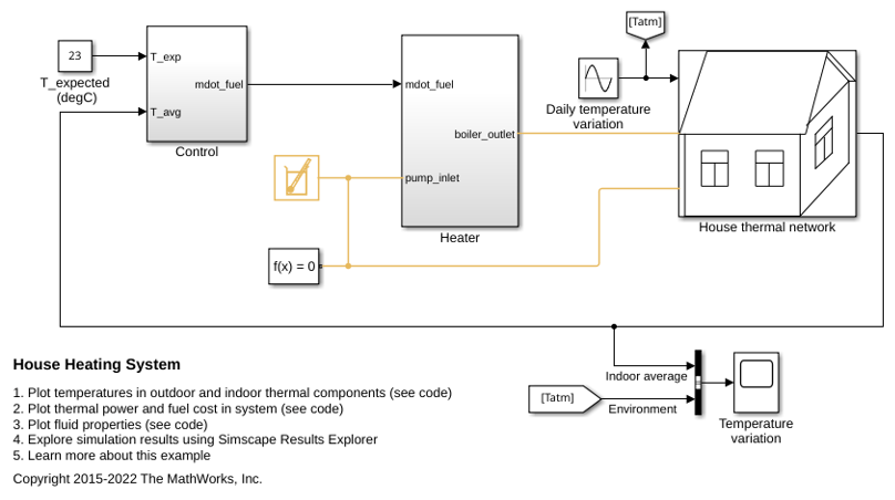
Model a simple house heating system. The model contains a heater, a controller, and a house structure with four radiators and four rooms. Each room exchanges heat with the environment through its exterior walls, roof, and windows. Each path is simulated as a combination of a thermal convection, thermal conduction, and the thermal mass. It is assumed that heat is not transferred internally between rooms. The heater consists of a furnace, a boiler, an accumulator, and a pump to circulate hot water in the system. The controller starts admitting fuel into the furnace if the overall average temperature of rooms falls below 21 degree C and it stops if the temperature exceeds 25 degree C. The simulation calculates the heating cost and indoor temperatures.
Electric Vehicle Thermal Management
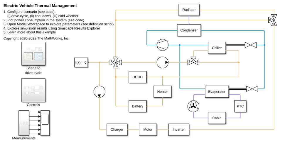
Model the thermal management system of a battery electric vehicle.
Pressure Loss and Mass Flow Rate in a Thermal Liquid Pipe
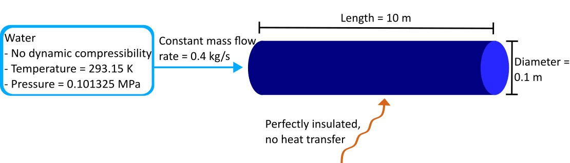
How changes in pipe and fluid attributes, such as friction and elevation change, impact the pressure loss through a pipe and how enabling dynamic compressibility impacts the mass flow rate. These effects are especially important in long, narrow pipes because they ensure the flow pressure is strong enough to overcome the pressure loss. This example uses the Simscape™ Fluids™ Pipe (TL) block.
Ports
Input
Conserving
Parameters
Algorithms
When the flow is laminar and Heat transfer parameterization is
Gnielinski correlation, Nominal temperature
differential vs. nominal mass flow rate, or
Dittus-Boelter correlation - Nusselt = a * Re^b * Pr^c,
the block determines the Nusselt number by using a lookup table and Nusselt number data
from [1],
[6], and
[7]. When
the block uses a lookup table, it uses linear interpolation and nearest extrapolation to
determine the Nusselt number.
The data that the block uses depends on the Cross-sectional geometry setting:
When Cross-sectional geometry is
Circular, the Nusselt number is 3.66.When Cross-sectional geometry is
Annular, the block calculates the Nusselt number from tabulated data.If Heat transfer walls is
Inner wall:Nusselt number 0.02 32.337 0.05 17.46 0.1 11.56 0.25 7.371 0.5 5.738 1 4.861 If Heat transfer walls is
Outer wall:Nusselt number 0 3.657 0.02 3.993 0.05 4.056 0.1 4.113 0.25 4.232 0.5 4.429 1 4.861 If Heat transfer walls is
Inner and outer walls:Nusselt Number Inner Wall Nusselt Number Outer Wall 0.0001 2355.3 2.779 0.001 322.254 2.823 0.01 50.454 2.908 0.02 30.179 2.948 0.04 18.614 2.999 0.05 16.058 3.019 0.06 14.28 3.036 0.08 11.943 3.068 0.1 10.459 3.095 0.15 8.342 3.157 0.2 7.197 3.213 0.25 6.471 3.267 0.3 5.966 3.319 0.4 5.305 3.421 0.5 4.889 3.52 0.6 4.602 3.619 0.7 4.391 3.715 0.8 4.23 3.811 0.9 4.103 3.906 1 4 4
When Cross-sectional geometry is
Rectangular, the block calculates the Nusselt number from tabulated data.Nusselt number 0 7.54 1/8 5.60 1/6 5.14 1/4 4.44 1/3 3.96 1/2 3.39 1 2.98 When Cross-sectional geometry is
Elliptical, the block calculates the Nusselt number from tabulated data.Nusselt number 1/16 3.65 1/8 3.72 1/4 3.79 1/2 3.74 1 3.66 When Cross-sectional geometry is
Isosceles
                                    triangular
, the block calculates the Nusselt number from tabulated data.θ Nusselt number 10π/180 1.61 30π/180 2.26 60π/180 2.47 90π/180 2.34 120π/180 2.00 When Cross-sectional geometry is
Custom, the Nusselt number is the value of the Nusselt number for laminar flow heat transfer parameter.
References
[1] Budynas R. G. Nisbett J. K. and Shigley J. E., 2004. Shigley's mechanical engineering design (7th ed.). McGraw-Hill.
[2] Cengel, Y.A. Heat and Mass Transfer: A Practical Approach (3rd edition). New York, McGraw-Hill, 2007
[3] Ju, Frederick D., and Thomas A. Butler. Review of proposed failure criteria for ductile materials. No. NUREG/CR-3644; LA-10007-MS. Los Alamos National Lab., NM (USA), 1984.
[4] Hencky, Heinrich. "Zur Theorie plastischer Deformationen und der hierdurch im Material hervorgerufenen Nachspannungen." ZAMM‐Journal of Applied Mathematics and Mechanics/Zeitschrift für Angewandte Mathematik und Mechanik 4, no. 4 (1924): 323-334.
[5] Jahed H., 1997. "A Variable Material Property Approach for Elastic-Plastic Analysis of Proportional and Non-proportional Loading". University of Waterloo
[6] Shah, Ramesh K., and Alexander Louis London. Laminar flow forced convection in ducts: a source book for compact heat exchanger analytical data. Academic press, 2014.
[7] Hirbodi, Kamran, Mahmood Yaghoubi, and David Martin Warsinger. "New Nusselt number correlations for developing and fully developed laminar flows in concentric circular annular ducts." International Communications in Heat and Mass Transfer 134 (2022): 105936.
[8] Petukhov, Boris Sergeevich, and Lev Ionovich Roizen. "Generalized relationships for heat transfer in turbulent flow of gas in tubes of annular section." Teplofizika vysokikh temperatur 2, no. 1 (1964): 78-81.
[9] Gnielinski, Volker. "Heat transfer coefficients for turbulent flow in concentric annular ducts." Heat transfer engineering 30, no. 6 (2009): 431-436.

