Solve a Mixed-Integer Engineering Design Problem Using the Genetic Algorithm, Problem-Based

This example shows how to solve a mixed-integer engineering design problem using the genetic algorithm (ga) solver in Global Optimization Toolbox. The example uses the problem-based approach. For a version using the solver-based approach, see Solve a Mixed-Integer Engineering Design Problem Using the Genetic Algorithm.

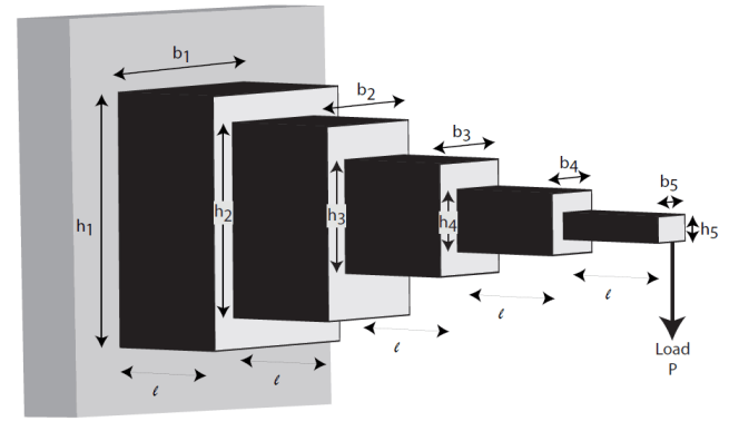
The problem illustrated in this example involves the design of a stepped cantilever beam. In particular, the beam must be able to carry a prescribed end load. The optimization problem is to minimize the beam volume subject to various engineering design constraints.

This problem is described in Thanedar and Vanderplaats [1].

Stepped Cantilever Beam Design Problem

A stepped cantilever beam is supported at one end, and a load is applied at the free end, as shown in the following figure. The beam must be able to support the given load $$P$$ at a fixed distance $$L$$ from the support. Designers of the beam can vary the width ($$b_i$$) and height ($$h_i$$) of each step, or section. Each section of the cantilever has the same length, $$l=L_1$$.

Volume of the Beam

The volume of the beam $$V$$ is the sum of the volume of the individual sections.

$$V=l(b_1{h}_1+b_2{h}_2+b_3{h}_3+b_4{h}_4+b_5{h}_5)$$.

Constraints on the Design: Bending Stress

Consider a single cantilever beam, with the center of coordinates at the center of its cross section at the free end of the beam. The bending stress at a point $$(x,y,z)$$ in the beam is given by the equation

$${\sigma }_b=M(x)y/I$$,

where $$M(x)$$ is the bending moment at $$x$$, $$x$$ is the distance from the end load, and $$I$$ is the area moment of inertia of the beam.

In the stepped cantilever beam shown in the figure, the maximum moment of each section of the beam is $$P{D}_i$$, where $$D_i$$ is the maximum distance from the end load $$P$$ for each section of the beam. Therefore, the maximum stress for the ith section of the beam $${\sigma }_i$$ is given by

$${\sigma }_i=P{D}_i(h_i/2)/I_i$$,

where the maximum stress occurs at the edge of the beam, $$y=h_i/2$$. The area moment of inertia of the ith section of the beam is given by

$$I_i=b_i{h}_i^3/12$$.

Substituting this expression into the equation for $${\sigma }_i$$ gives

$${\sigma }_i=6P{D}_i/b_i{h}_i^2$$.

The bending stress in each part of the cantilever must not exceed the maximum allowable stress $${\sigma }_{max}$$. Therefore, the five bending stress constraints (one for each step of the cantilever) are:

$$\frac{6Pl}{b_5{h}_5^2}\le {\sigma }_{max}$$

$$\frac{6P(2l)}{b_4{h}_4^2}\le {\sigma }_{max}$$

$$\frac{6P(3l)}{b_3{h}_3^2}\le {\sigma }_{max}$$

$$\frac{6P(4l)}{b_2{h}_2^2}\le {\sigma }_{max}$$

$$\frac{6P(5l)}{b_1{h}_1^2}\le {\sigma }_{max}$$

Constraints on the Design: End Deflection

You can calculate the end deflection of the cantilever using Castigliano's second theorem, which states that

$$\delta =\frac{\partial U}{\partial P}$$,

where $$\delta$$ is the deflection of the beam, and $$U$$ is the energy stored in the beam due to the applied force $$P$$.

The energy stored in a cantilever beam is given by

$$U={\int }_0^L{M}^2/2EIdx$$,

where $$M$$ is the moment of the applied force at $$x$$.

Given that $$M=Px$$ for a cantilever beam, you can write the preceding equation as

$$U=P^2/2E{\int }_0^l[(x+4l{)}^2/I_1+(x+3l{)}^2/I_2+(x+2l{)}^2/I_3+(x+l{)}^2/I_4+x^2/I_5]dx$$,

where $$I_n$$ is the area moment of inertia of the nth part of the cantilever. Evaluating the integral gives this expression for $$U$$

$$U=(P^2/2)(l^3/3E)(61/I_1+37/I_2+19/I_3+7/I_4+1/I_5)$$.

Applying Castigliano's theorem, the end deflection of the beam is given by

$$\delta =P{l}^3/3E(61/I_1+37/I_2+19/I_3+7/I_4+1/I_5)$$.

The end deflection of the cantilever $$\delta$$ must be less than the maximum allowable deflection $${\delta }_{max}$$, which gives the constraint

$$P{l}^3/3E(61/I_1+37/I_2+19/I_3+7/I_4+1/I_5)\le {\delta }_{max}$$.

Constraints on the Design: Aspect Ratio

For each step of the cantilever, the aspect ratio must not exceed a maximum allowable aspect ratio $$a_{max}$$. That is,

$$h_i/b_i\le a_{max}$$ for $$i=1,...,5$$.

Constraints on the Design: Bounds and Integer Constraints

The first step of the beam can be machined to the nearest centimeter only. That is, $$b_1$$ and $$h_1$$ must be integers. The remaining variables are continuous. The bounds on the variables are:

$$1\le b_1\le 5$$

$$30\le h_1\le 65$$

$$2.4\le b_2,b_3\le 3.1$$

$$45\le h_2,h_3\le 60$$

$$1\le b_4,b_5\le 5$$

$$30\le h_4,h_5\le 65$$

Design Parameters for This Problem

For the problem in this example, the end load that the beam must support is $$P=50000N$$.

The beam lengths and maximum end deflection are:

• Total beam length, $$L=500cm$$

• Length of an individual section of the beam, $$l=L_1=100cm$$

• Maximum beam end deflection, $${\delta }_{max}=2.7cm$$

The maximum allowed stress in each step of the beam is $${\sigma }_{max}=14000N/c{m}^2$$.

Young's modulus of each step of the beam is $$E=2\times 10^{7}N/c{m}^2$$.

Problem-Based Setup

Create optimization variables for this problem. The width and height variables for the first section of the beam are of type integer, so you must create them separately from the other four variables, which are continuous.

b1 = optimvar("b1","Type","integer","LowerBound",1,"UpperBound",5);
h1 = optimvar("h1","Type","integer","LowerBound",30,"UpperBound",65);
bc = optimvar("bc",4,"LowerBound",[2.4 2.4 1 1],"UpperBound",[3.1 3.1 5 5]);
hc = optimvar("hc",4,"LowerBound",[45 45 30 30],"UpperBound",[60 60 65 65]);

For convenience, put the height and width variables into single variables. You can then express the objective and constraints easily in terms of these variables.

h = [h1;hc];
b = [b1;bc];

Create an optimization problem with the volume of the beam as the objective function, where each step (or section) of the beam is $$L_1=100$$ cm long: volume = $$L_1\sum h_i{w}_i$$.

L_1 = 100; % Length of each step of the cantilever
prob = optimproblem("Objective",L_1*dot(h,b));

Create the constraints on the stress.

P = 50000; % End load
E = 2e7; % Young's modulus in N/cm^2
deltaMax = 2.7; % Maximum end deflection
sigmaMax = 14000; % Maximum stress in each section of the beam
aMax = 20; % Maximum aspect ratio in each section of the beam

stress = 6*P*L_1./(b.*(h.^2));
stepnum = (5:-1:1)';
stress = stress.*stepnum;
prob.Constraints.stress = stress <= sigmaMax;

Create the constraint on the deflection.

deflectionMultiplier = (P*L_1^3/E)*[244 148 76 28 4];
bh3 = 1./(b.*(h.^3));
prob.Constraints.deflection = deflectionMultiplier*bh3 <= deltaMax;

Create the constraints on the aspect ratio.

prob.Constraints.aspect = h <= aMax*b;

Review the problem setup.

show(prob)

  OptimizationProblem : 

	Solve for:
       b1, bc, h1, hc
	where:
       b1, h1 integer

	minimize :
       100*h1*b1 + 100*hc(1)*bc(1) + 100*hc(2)*bc(2) + 100*hc(3)*bc(3) + 100*hc(4)*bc(4)


	subject to stress:
       arg_LHS <= arg_RHS

       where:

             arg2 = zeros(5, 1);
             arg1 = zeros(5, 1);
             arg1(1) = h1;
             arg1(2:5) = hc;
             arg2(1) = b1;
             arg2(2:5) = bc;
             arg_LHS = ((30000000 ./ (arg2(:) .* arg1(:).^2)) .* extraParams{1});
             arg2 = 14000;
             arg1 = arg2(ones(1,5));
             arg_RHS = arg1(:);

         extraParams{1}:

          5
          4
          3
          2
          1




	subject to deflection:
       arg_LHS <= 2.7

       where:

             arg2 = zeros(5, 1);
             arg1 = zeros(5, 1);
             arg1(1) = h1;
             arg1(2:5) = hc;
             arg2(1) = b1;
             arg2(2:5) = bc;
             arg_LHS = (extraParams{1} * (1 ./ (arg2(:) .* arg1(:).^3)));

         extraParams{1}:

           610000      370000      190000       70000       10000




	subject to aspect:
       -20*b1 + h1 <= 0
       -20*bc(1) + hc(1) <= 0
       -20*bc(2) + hc(2) <= 0
       -20*bc(3) + hc(3) <= 0
       -20*bc(4) + hc(4) <= 0

	variable bounds:
       1 <= b1 <= 5

       2.4 <= bc(1) <= 3.1
       2.4 <= bc(2) <= 3.1
         1 <= bc(3) <= 5
         1 <= bc(4) <= 5

       30 <= h1 <= 65

       45 <= hc(1) <= 60
       45 <= hc(2) <= 60
       30 <= hc(3) <= 65
       30 <= hc(4) <= 65

Solve the Problem

Set options to use a moderate population size of 150, a moderate maximum number of generations of 400, a slightly larger than default elite count of 10, a small function tolerance of 1e-8, and a plot function showing the function value during the iterations.

opts = optimoptions(@ga, ...
                    'PopulationSize', 150, ...
                    'MaxGenerations', 400, ...
                    'EliteCount', 10, ...
                    'FunctionTolerance', 1e-8, ...
                    'PlotFcn', @gaplotbestf);

Solve the problem, specifying the ga solver and the options.

rng default % For reproducibility
[sol,fval,exitflag] = solve(prob,"Solver","ga","Options",opts)

Solving problem using ga.

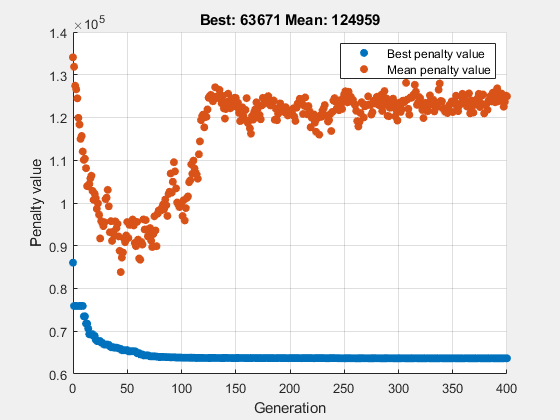
ga stopped because the average change in the penalty function value is less than options.FunctionTolerance and 
the constraint violation is less than options.ConstraintTolerance.

sol = struct with fields:
    b1: 3
    bc: [4x1 double]
    h1: 60
    hc: [4x1 double]

fval = 
6.3804e+04

exitflag = 
    SolverConvergedSuccessfully

View the solution variables and their bounds.

widths = [sol.b1;sol.bc];
heights = [sol.h1;sol.hc];
widthbounds = [b1.LowerBound b1.UpperBound;
    bc.LowerBound bc.UpperBound];
heightbounds = [h1.LowerBound h1.UpperBound;
    hc.LowerBound hc.UpperBound];
T = table(widths,heights,widthbounds,heightbounds,...
    'VariableNames',["Width" "Height" "Width Bounds" "Height Bounds"])

T=5×4 table
    Width     Height    Width Bounds    Height Bounds
    ______    ______    ____________    _____________

         3        60       1      5       30    65   
    2.9063    54.983     2.4    3.1       45    60   
    2.5805    51.609     2.4    3.1       45    60   
    2.2785    45.565       1      5       30    65   
    1.7502    34.991       1      5       30    65   

The solution is not at any of the bounds. The first solution variables are integer valued, as specified.

Add Discrete Noninteger Variable Constraints

Suppose the engineers learn that the second and third steps of the cantilever can have widths and heights selected from a standard set only. With the addition of this constraint, the problem is identical to the one solved in [1].

First, delineate the extra constraints to add to the optimization:

• The width of the second and third steps of the beam must be selected from the set [2.4, 2.6, 2.8, 3.1] cm.

• The height of the second and third steps of the beam must be selected from the set [45, 50, 55, 60] cm.

To solve this problem, you need to specify the variables $$wc(1)$$, $$wc(2)$$, $$hc(1)$$, and $$hc(2)$$ as discrete variables. Ideally, you would use $$S(x_j)$$ as the discrete value, where $$S$$ represents the allowable set of values and $$x_j$$ represents a problem variable. However, you cannot use an optimization variable as an index. You can get around this problem by calling fcn2optimexpr.

widthlist = [2.4,2.6,2.8,3.1];
heightlist = [45 50 55 60];
b23 = optimvar("w23",2,"Type","integer",...
    "LowerBound",1,"UpperBound",length(widthlist));
h23 = optimvar("h23",2,"Type","integer",...
    "LowerBound",1,"UpperBound",length(heightlist));
b45 = optimvar("b45",2,"LowerBound",1,"UpperBound",5);
h45 = optimvar("h45",2,"LowerBound",30,"UpperBound",65);
% Preferred syntax is we = [widthlist(b23(1));widthlist(b23(2))];
% However, this syntax is illegal.
% Instead call fcn2optimexpr.
we = fcn2optimexpr(@(x)[widthlist(x(1));widthlist(x(2))],b23);
he = fcn2optimexpr(@(x)[heightlist(x(1));heightlist(x(2))],h23);

As you did earlier, create the expressions b and h to represent the variables.

b = [b1;we;b45];
h = [h1;he;h45];

The remainder of the problem formulation is the same as earlier.

prob2 = optimproblem("Objective",L_1*dot(h,b));

Create the constraints on the stress.

stress = 6*P*L_1./(b.*(h.^2));
stepnum = (5:-1:1)';
stress = stress.*stepnum;
prob2.Constraints.stress = stress <= sigmaMax;

Create the constraint on the deflection.

deflectionMultiplier = (P*L_1^3/E)*[244 148 76 28 4];
bh3 = 1./(b.*(h.^3));
prob2.Constraints.deflection = deflectionMultiplier*bh3 <= deltaMax;

Create the constraints on the aspect ratio.

prob2.Constraints.aspect = h <= aMax*b;

Review the problem setup.

show(prob2)

  OptimizationProblem : 

	Solve for:
       b1, b45, h1, h23, h45, w23
	where:
       b1, h1, h23, w23 integer

	minimize :
       (100 .* (arg2(:).' * arg4(:)))

       where:

           arg4 = zeros(5, 1);
           arg2 = zeros(5, 1);
           anonymousFunction2 = @(x)[heightlist(x(1));heightlist(x(2))];
           arg1 = anonymousFunction2(h23);
           arg2(1) = h1;
           arg2(2:3) = arg1;
           arg2(4:5) = h45;
           anonymousFunction1 = @(x)[widthlist(x(1));widthlist(x(2))];
           arg3 = anonymousFunction1(w23);
           arg4(1) = b1;
           arg4(2:3) = arg3;
           arg4(4:5) = b45;


	subject to stress:
       arg_LHS <= arg_RHS

       where:

             arg4 = zeros(5, 1);
             arg2 = zeros(5, 1);
             anonymousFunction2 = @(x)[heightlist(x(1));heightlist(x(2))];
             arg1 = anonymousFunction2(h23);
             arg2(1) = h1;
             arg2(2:3) = arg1;
             arg2(4:5) = h45;
             anonymousFunction1 = @(x)[widthlist(x(1));widthlist(x(2))];
             arg3 = anonymousFunction1(w23);
             arg4(1) = b1;
             arg4(2:3) = arg3;
             arg4(4:5) = b45;
             arg_LHS = ((30000000 ./ (arg4(:) .* arg2(:).^2)) .* extraParams{1});
             arg2 = 14000;
             arg1 = arg2(ones(1,5));
             arg_RHS = arg1(:);

         extraParams{1}:

          5
          4
          3
          2
          1




	subject to deflection:
       arg_LHS <= 2.7

       where:

             arg4 = zeros(5, 1);
             arg2 = zeros(5, 1);
             anonymousFunction2 = @(x)[heightlist(x(1));heightlist(x(2))];
             arg1 = anonymousFunction2(h23);
             arg2(1) = h1;
             arg2(2:3) = arg1;
             arg2(4:5) = h45;
             anonymousFunction1 = @(x)[widthlist(x(1));widthlist(x(2))];
             arg3 = anonymousFunction1(w23);
             arg4(1) = b1;
             arg4(2:3) = arg3;
             arg4(4:5) = b45;
             arg_LHS = (extraParams{1} * (1 ./ (arg4(:) .* arg2(:).^3)));

         extraParams{1}:

           610000      370000      190000       70000       10000




	subject to aspect:
       arg_LHS <= arg_RHS

       where:

             arg1 = zeros(5, 1);
             arg1(1) = h1;
             anonymousFunction2 = @(x)[heightlist(x(1));heightlist(x(2))];
             arg2 = anonymousFunction2(h23);
             arg1(2:3) = arg2;
             arg1(4:5) = h45;
             arg_LHS = arg1(:);
             arg2 = zeros(5, 1);
             anonymousFunction1 = @(x)[widthlist(x(1));widthlist(x(2))];
             arg1 = anonymousFunction1(w23);
             arg2(1) = b1;
             arg2(2:3) = arg1;
             arg2(4:5) = b45;
             arg_RHS = (20 .* arg2(:));

	variable bounds:
       1 <= b1 <= 5

       1 <= b45(1) <= 5
       1 <= b45(2) <= 5

       30 <= h1 <= 65

       1 <= h23(1) <= 4
       1 <= h23(2) <= 4

       30 <= h45(1) <= 65
       30 <= h45(2) <= 65

       1 <= w23(1) <= 4
       1 <= w23(2) <= 4

Solve the Problem with Discrete Variable Constraints

Solve the problem, specifying the ga solver and the options.

rng default % For reproducibility
[sol2,fval2,exitflag2] = solve(prob2,"Solver","ga","Options",opts)

Solving problem using ga.

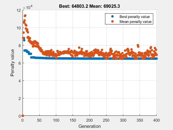
ga stopped because it exceeded options.MaxGenerations.

sol2 = struct with fields:
     b1: 3
    b45: [2x1 double]
     h1: 60
    h23: [2x1 double]
    h45: [2x1 double]
    w23: [2x1 double]

fval2 = 
6.4803e+04

exitflag2 = 
    SolverLimitExceeded

The objective value increases, because adding constraints can only increase the objective.

View the solution and compare it to its bounds.

widths = [sol2.b1;widthlist(sol2.w23(1));widthlist(sol2.w23(2));sol2.b45];
heights = [sol2.h1;heightlist(sol2.h23(1));heightlist(sol2.h23(2));sol2.h45];
widthbounds = [b1.LowerBound b1.UpperBound;
    widthlist(1) widthlist(end);
     widthlist(1) widthlist(end);
    b45.LowerBound b45.UpperBound];
heightbounds = [h1.LowerBound h1.UpperBound;
     heightlist(1) heightlist(end);
     heightlist(1) heightlist(end);
    h45.LowerBound h45.UpperBound];
T = table(widths,heights,widthbounds,heightbounds,...
    'VariableNames',["Width" "Height" "Width Bounds" "Height Bounds"])

T=5×4 table
    Width     Height    Width Bounds    Height Bounds
    ______    ______    ____________    _____________

         3        60       1      5       30    65   
       3.1        55     2.4    3.1       45    60   
       2.6        50     2.4    3.1       45    60   
     2.286     45.72       1      5       30    65   
    1.8532    34.004       1      5       30    65   

The only solution variable that is at a bound is the width of the second section, which is 3.1, its maximum.

References

[1] Thanedar, P. B., and G. N. Vanderplaats. "Survey of Discrete Variable Optimization for Structural Design." Journal of Structural Engineering 121 (3), 1995, pp. 301–306.