Track Closely Spaced Targets Under Ambiguity in Simulink
This example shows how to track objects in Simulink® with Sensor Fusion and Tracking Toolbox™ when the association of sensor detections to tracks is ambiguous. It closely follows the Tracking Closely Spaced Targets Under Ambiguity MATLAB® example.
Introduction
Sensors report a single detection for multiple targets when the targets are so closely spaced that the sensors cannot resolve them spatially. This example illustrates the workflow for tracking targets under such ambiguity using the global nearest neighbor (GNN), joint probabilistic data association (JPDA), and track-oriented multiple-hypothesis (TOMHT) trackers.
Setup and Overview of the Model
Prior to running this example, the scenario was generated as described in Tracking Closely Spaced Targets Under Ambiguity. The detection and time data from this scenario were then saved to the scenario file CloselySpacedData.mat.
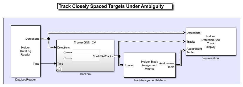
DataLogReader
The DataLogReader block is implemented as a MATLAB System (Simulink) block. The code for the block is defined by a helper class, HelperDataLogReader. The block reads the recorded data from the CloselySpacedData.mat file and outputs the detection and time for each time stamp.
Trackers
The Trackers block is a variant subsystem block, which has six subsystems defined internally. Each subsystem is composed of one of the three trackers and one of the two motion models.
![]()
The first motion model is a constant velocity model with an extended kalman filter. The helperCVFilter function modifies the filter initcvekf returns to allow for a higher uncertainty in the velocity terms and a higher horizontal acceleration in the process noise.
The second filter you use is an interacting multiple-model (IMM) filter, which allows you to define two or more motion models for the targets. The filter automatically updates the likelihood of each motion model based on the give measurements and estimates the target state and uncertainty based on these models and likelihoods. In this example, the targets switch between straight legs at a constant velocity motion and legs of constant turn rate. Therefore, you define an IMM filter with a constant velocity model and a constant turn-rate model using the helperIMMFilter function.
You can run the different configurations by changing the value of Tracker in the workspace as shown in the above table. You can also use the Edit and Manage Workspace Variables by Using Model Explorer (Simulink) as shown below to change the value of Tracker.
![]()
TrackAssignmentMetrics
The TrackAssignmentMetrics is implemented using a MATLAB System (Simulink) block. The code for the block is defined by a helper class, HelperTrackAssignmentMetrics.
Visualization
The visualization block is implemented using a MATLAB System (Simulink) block. The code for the block is defined by a helper class, HelperDetectionAndTrackDisplay.
Detections and Tracks Bus Objects
The trackers variant subsystem block receives the detections as a bus object with time values and outputs the tracks as a bus object to the visualization block. You can visualize the structure of each bus using the Type Editor (Simulink). The following images show the structure of the bus for detections and tracks.
Detections Bus
The detectionBus outputs a nested bus object with 2 elements, NumDetections and Detections.

The first element Detections is a fixed-size bus object representing all detections. The second element, NumDetections, represents the number of detections. The structure of the bus is similar to the objectDetection class.

Tracks Bus
The track bus is similar to the detections bus. The track bus is a nested bus, where NumTracks defines the number of tracks in the bus and Tracks define a fixed size of tracks. The size of the tracks is governed by the block parameter Maximum number of tracks. The figure below shows the configuration of the tracks bus object for trackerGNN. The configuration of the tracks bus object for trackerJPDA and trackerTOMHT is similar.
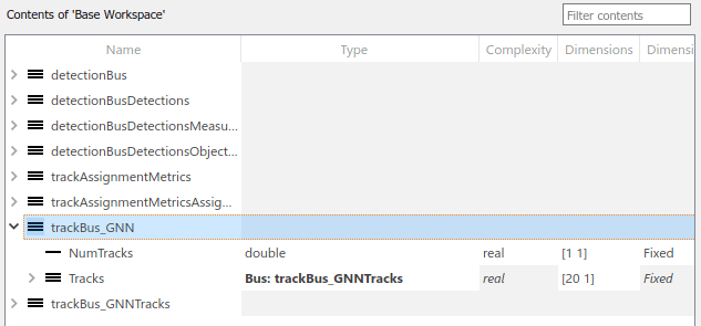
The second element Tracks is a bus object defined by trackBus_GNNTracks for the trackerGNN configuration. This bus is automatically created by the tracker block using the bus name specified as the prefix. The structure of the bus is similar to the objectTrack class.

Results
Tracker configuration in the Trackers variant subsystem block is similar to that of the Tracking Closely Spaced Targets Under Ambiguity MATLAB® example.
You can run the trackerGNN, trackerJPDA, and trackerTOMHT blocks in Simulink® models via interpreted execution or code generation. With interpreted execution, the model simulates the block using the MATLAB® execution engine which allows faster startup time but longer execution time. With code generation, the model uses the subset of MATLAB code supported for code generation which allows better performance than the interpreted execution.
After running the model you can visualize the results on the figures.
![]()
The above results are achieved from the first configuration where Tracker = 1 in MATLAB workspace. These results show that there are two truth objects. However, the tracker generate three confirmed tracks, and one of the tracks did not survive until the end of the scenario. At the end of the scenario, the tracker associates truth object 1 with track 8. The tracker created track 8 through the scenario after dropping track 2. The tracker assigned truth object 2 to track 1 at the end of the scenario after there were two track breaks in the tracking history.
![]()
The above results are achieved from the second configuration where Tracker = 2 in MATLAB workspace. The IMM filter enables the trackerGNN to track the maneuvering target correctly. Notice that truth object 1 has zero breaks due to continuous history of its associated track.
However, even with the IMM filter, one of the tracks breaks in the ambiguity region. The trackerGNN receives only one detection in that ambiguity region, and therefore can update only one of the tracks with it. After a few updates, the score of the coasted track falls below the deletion threshold and the tracker drops the track.
![]()
The above results are achieved from the third configuration where Tracker = 3 in MATLAB workspace. You can observe that the trackerJPDA maintains both the tracks confirmed in the ambiguity region. However, there is a swap between the two tracks.
![]()
The above results are achieved from the fourth configuration where Tracker = 4 in MATLAB workspace. You can observe that trackerJPDA with IMM filter tracks the maneuvering targets more precisely and did not break or lose the track even during the turns.
![]()
Next, the fifth configuration is used, with trackerTOMHT and a constant velocity model by setting Tracker = 5 in MATLAB workspace. You can observe that the trackerTOMHT result is similar to the one obtained by the trackerJPDA: it maintains the tracks through the ambiguity region, but relying only on a constant velocity model causes the tracks to swap.
![]()
Finally, we use trackerTOMHT and IMM filter by setting Tracker = 6 in MATLAB workspace. This time, the trackerTOMHT with IMM filter tracks the maneuvering targets more precisely and did not break or lose the track even during the turns. However, the runtime for a trackerTOMHT is significantly longer than using trackerJPDA.
Summary
In this example, you learned how to track closely spaced targets using three types of trackers: global nearest neighbor, joint probabilistic data association, and track-oriented multiple hypothesis. You saw how to use a variant subsystem in Simulink to select which tracker and filter to run. You also learned how you can utilize and configure trackerGNN, trackerJPDA, and trackerTOMHT Simulink blocks for tracking the maneuvering targets.
You observed that a constant velocity filter is insufficient when tracking the targets during their maneuver. In this case, an interacting multiple-model filter is required. You also observed that the JPDA and TOMHT trackers can more accurately handle the case of ambiguous association of detections to tracks compared with the GNN tracker.