Use the Fixed-Point Tool to Rescale a Fixed-Point Model
This example show you how to use the Fixed-Point Tool to refine the scaling of fixed-point data types associated with the feedback controller model fxpdemo_feedback. The Fixed-Point Tool enables multiple workflows for converting a model to use fixed-point data types.
The Range Collection workflow in the Fixed-Point Tool allows you to explore the numerical behavior of your model before or after data type conversion.
The Iterative Fixed-Point Conversion workflow in the Fixed-Point Tool automates common tasks of collecting min-max range data during simulations for use in automatically selecting fixed-point data types for blocks. You can configure any fixed-point capable block in Simulink® to accept the fixed-point data types proposed by the tool. You can manually specify data types for key blocks such as input ports and selectively disable automated scaling in a model on a block-by-block basis. This gives the Fixed-Point Tool more information to work with and results in automatically selected fixed-point scalings that are compatible with the key manually selected scalings.
This example uses the following approach:
Range Collection - Use the range collection workflow to explore the numerical behavior of the model. Run an initial simulation using a reasonable guess at the fixed-point word size and scaling. Then override data types in the model with double-precision numbers and compare the simulation results.
Iterative Fixed-Point Conversion - Propose fraction lengths for using double-precision simulation range data. The Fixed-Point Tool allows you to selectively accept and apply the scaling proposals, then verify the quality of the results by simulating the model with applied data types.
Open Feedback Controller Model
The fxpdemo_feedback model contains a digital controller with initial guesses for fixed-point data types already specified in the Controller subsystem. In this example, you specify a known tolerance for the plant output, propose new fixed-point data types for the Controller subsystem, then apply the proposed data types to the model.
open_system('fxpdemo_feedback')
The model consists of these blocks and subsystems:
Reference - This Signal Generator block generates a continuous-time reference signal. It is configured to output a square wave.
Sum - This Add block subtracts the plant output from the reference signal.
ZOH - The Zero-Order Hold block samples and holds the continuous signal. This block is configured so that it quantized the signal in time by 0.01 seconds.
Analog to Digital Interface - The analog to digital (A/D) interface consists of a Data Type Conversion block that converts a double to a fixed-point data type. It represents any hardware that digitizes the amplitude of the analog input signal. In the real world, its characteristics are fixed.
Controller - The digital controller is a subsystem that represents the software running on the hardware target.
Digital to Analog Interface - The digital to analog (D/A) interface consists of a Data Type Conversion block that converts a fixed-point data type into a double. It represents any hardware that converts a digitized signal into an analog signal. In the real world, its characteristics are fixed.
Analog Plant - The analog plant is described by a transfer function and is controlled by the digital controller. In the real world, its characteristics are fixed.
Scope - The model includes a Scope block that displays the plant output signal.
Simulation Setup
To set up this kind of fixed-point feedback controller simulation:
Identify all design components. In the real world, there are design components with fixed characteristics (the hardware) and design components with characteristics that you can change (the software). In this feedback design, the main hardware components are the A/D hardware, the D/A hardware, and the analog plant. The main software component is the digital controller.
Develop a theoretical model of the plant and controller. For the feedback design in this tutorial, the plant is characterized by a transfer function. The digital controller model in this tutorial is described by a z-domain transfer function and is implemented using a direct-form realization.
Evaluate the behavior of the plant and controller. You evaluate the behavior of the plant and the controller with a Bode plot. This evaluation is idealized, because all numbers, operations, and states are double-precision.
Simulate the system. Simulate the feedback controller design using Simulink and the Fixed-Point Designer™ software. In a simulation environment, you can treat all components (software and hardware) as though their characteristics are not fixed.
Idealized Feedback Design
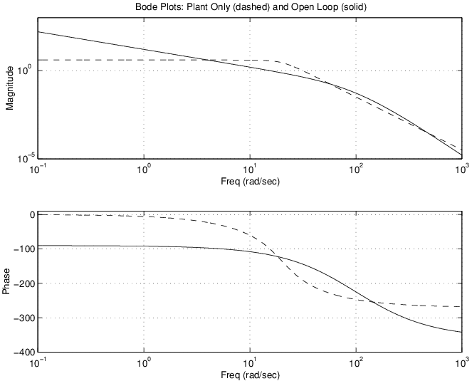
Open loop (controller and plant) and plant-only Bode plots for the model are shown in the following figure. The open loop Bode plot results from a digital controller described in the idealized world of continuous time, double-precision coefficients, storage of states, and math operations. The Bode plots were created using workspace variables produced by the preload_feedback script.
Digital Controller Realization
In this model, the digital controller is implemented using the fixed-point direct form realization shown in the following diagram. The hardware target is a 16-bit processor. Variables and coefficients are generally represented using 16 bits, especially if these quantities are stored in ROM or global RAM. Use of 32-bit numbers is limited to temporary variables that exist briefly in CPU registers or in a stack.

The digital controller realization consists of these blocks:
Up Cast - This Data Type Conversion block connects the A/D hardware with the digital controller. It pads the output word size of the A/D hardware with trailing zeros to a 16-bit number (the base data type).
Numerator Terms and Denominator Terms - Each of these Discrete FIR Filter blocks represents a weighted sum carried out in the CPU target. The word size and precision in the calculations reflect those of the accumulator. Numerator Terms multiplies and accumulates the most recent inputs with the FIR numerator coefficients. Denominator Terms multiples and accumulates the most recent delayed outputs with the FIR denominator coefficients. The coefficients are stored in ROM using the base data type. The most recent inputs are stored in global RAM using the base data type.
Combine Terms - This Add block represents the accumulator in the CPU. Its word size and precision are twice that of the RAM (double bits).
Down Cast - This Data Type Conversion block represents taking the number from the CPU and storing it in RAM. The word size and precision are reduced to half that of the accumulator when converted back to the base data type.
Prev Out - This Unit Delay block delays the feedback signal in memory by one sample period. The signals are stored in global RAM using the base data type.
Direct Form Realization
The controller directly implements this equation:

where:
u**(k – 1)** represents the input from the previous time step.
y**(k) represents the current output, and y(k – 1)** represents the output from the previous time step.
bi represents the FIR numerator coefficients.
ai represents the FIR denominator coefficients.
The first summation in y**(k) represents the multiplication and accumulation of the most recent inputs and numerator coefficients in the accumulator. The second summation in y(k)** represents the multiplication and accumulation of the most recent outputs and denominator coefficients in the accumulator. Because the FIR coefficients, inputs, and outputs are all represented by 16-bit numbers (the base data type), any multiplication involving these numbers produces a 32-bit output (the accumulator data type).
Open Fixed-Point Tool
On the Simulink Apps tab, under Code Generation, click the Fixed-Point Tool icon.
Explore Numerical Behavior of Model
Initial guesses for the scaling of each block are already specified in each block mask in the model. Use the Range Collection workflow in the Fixed-Point Tool to compare the behavior of the model with an idealized double-precision floating-point version.
In the Fixed-Point Tool, select New > Range Collection.
Under System Under Design (SUD), select the subsystem you want to analyze. For this example, select Controller.
Under Range Collection Mode, select Simulation ranges.
Under Simulation Inputs, select Use default model inputs.
Click the Collect Ranges button arrow and select Double precision. Click the Collect Ranges button to start the range collection simulation. The software simulates the
fxpdemo_feedbackmodel in the double-precision data type override mode and stores the results inBaselineRun. Data type override enables you to perform a global override of the fixed-point data types, thereby avoiding quantization effects. The results of the run are displayed in the Results spreadsheet. The compiled data type (CompiledDT) column forBaselineRunshows that the blocks in the model used adoubledata type during simulation.Next, simulate the system using the fixed-point data types specified in the model. Click the Settings button arrow and select Specified data types. Click the Simulate with Embedded Types button. The software simulates the model using the currently specified fixed-point data types and stores the range information in
EmbeddedRun. You can view the collected ranges in the SimMin and SimMax columns of the spreadsheet.The Fixed-Point Tool highlights the row containing the Up Cast block to indicate that there is an issue with this result. Select the Up Cast row in the spreadsheet. The Result Details pane shows that the block saturated 23 times, which indicates a poor guess for its scaling. You can use the Explore tab in the Fixed-Point Tool to further explore and filter results.
Click Compare Results to compare the results in the Simulation Data Inspector.
In the Simulation Data Inspector, select
PlantOutputas the signal to compare. The Simulation Data Inspector plots the signal associated with the plant output forBaslineRunandEmbeddedRun. The plot of the plant output signal forEmbeddedRunreflects the initial guess at scaling. The Bode plot design sought to produce a well-behaved linear response for the closed-loop system, represented by the idealBaselineRun. However, the response of theEmbeddedRunis nonlinear. Significant quantization effects cause the nonlinear features. An important part of fixed-point design is finding a scaling that reduces quantization effects to acceptable levels.

Propose Fraction Lengths Using Simulation Range Data
Using automatic data typing, you can maximize the precision of the output data type while spanning the full simulation range. The iterative fixed-point conversion workflow in the Fixed-Point Tool lets you maximize the precision of the output data types while spanning the full simulation range. This process is known as autoscaling. Because no design range information is supplied in this example, the Fixed-Point Tool uses simulation range data for proposing data types. When the maximum and minimum simulation values cover the full, intended operating range of your design, the Fixed-Point Tool yields meaningful automatic data typing results.
Set Up Model for Conversion to Fixed-Point
Next, set up the fixed-point conversion workflow. Note that switching workflows in the Fixed-Point Tool clears the settings and any data collected during the active workflow. The model remains in its current state.
Start the iterative fixed-point conversion workflow. In the Fixed-Point Tool, select New > Iterative Fixed-Point Conversion.
Select the subsystem that you want to convert. Under System Under Design (SUD), select the
Controllersubsystem.Choose the range collection method to use. Under Range Collection Mode, select Simulation ranges.
Specify Simulation Inputs. For this example, use the default model inputs for simulation.
Specify signal tolerances for logged signals. Set the Absolute Tolerance of the
Plant Outputsignal to0.1.

Prepare Model for Conversion to Fixed Point
To prepare the model for fixed-point conversion, click Prepare. The Fixed-Point Tool creates a backup version of the model and checks the model for compatibility with the conversion process. For more information about preparation checks, see Use the Fixed-Point Tool to Prepare a System for Conversion.

Collect Ranges
To collect ranges, click the Collect Ranges button arrow and select Double precision. Click Collect Ranges to start the range collection simulation.

When you select Double precision as the range collection mode, the tool simulates the fxpdemo_feedback model with data type override enabled. Data type override performs a global override of the fixed-point data types in the model, thereby avoiding quantization effects. This enables you to establish an ideal floating-point baseline for the behavior of your model.
The results of range collection are stored in BaselineRun. The Results spreadsheet displays a summary of the statistics collected during the range collection simulation, including the currently specified data types on the model (SpecifiedDT), simulation minimum, and simulation maximum values. The compiled data type (CompiledDT) column displays double for all objects in the Controller subsystem, indicating that data type override was applied during the range collection simulation.
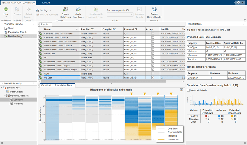
You can click any result to view additional details in the Results Details pane. The Visualization of Simulation Data pane displays a summary of histograms of the bits used by each object in your model. You can customize the information displayed in the Results spreadsheet, or use the Explore tab to sort and filter these results based on additional criteria. For more information, see Control Views in the Fixed-Point Tool.

Propose Fixed-Point Data Types
To configure the settings to use for data type proposals, expand the Settings button arrow. Set the Safety margin for simulation min/max (%) parameter to 20. Use the default settings for all other parameters.
The Safety margin for simulation min/max (%) parameter value multiplies the “raw” simulation values. Setting this parameter to a value greater than 1 decreases the likelihood that an overflow will occur when fixed-point data types are being used. Because of the nonlinear effects of quantization, a fixed-point simulation produces results that are different from an idealized, doubles-based simulation. Signals in a fixed-point simulation can cover a larger or smaller range than in a doubles-based simulation. If the range increases enough, overflows or saturations could occur. A safety margin decreases this likelihood, but it might also decrease the precision of the simulation.
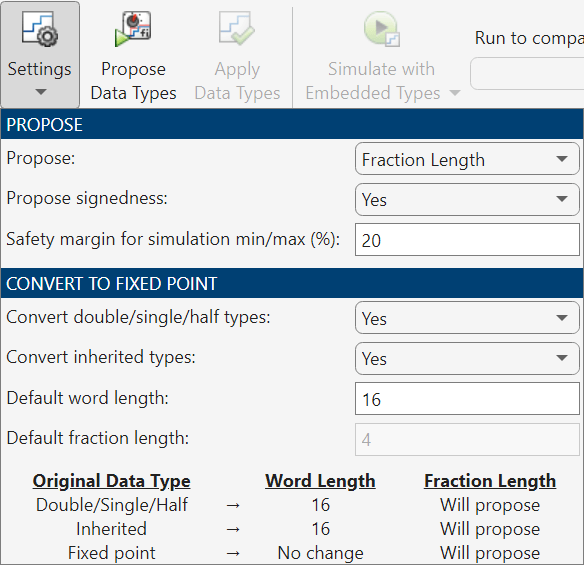
To propose data types based on the ranges collected and the data type proposal settings specified, click Propose Data Types. The tool uses all available range data to calculate data type proposals which can include design minimum or maximum values, simulation minimum or maximum values, and derived minimum or maximum values. Data types are proposed for all objects in the system under design whose Lock output data type setting against changes by the fixed-point tools parameter is cleared.
The Results spreadsheet updates to show the proposed data types in the ProposedDT column. The Fixed-Point Tool allows you to selectively apply data type proposals to objects in your model. In the spreadsheet, use the Accept check boxes to specify the proposed data types that you want to apply to your model. By default, the app accepts all data type proposals which differ from the currently specified data types. For this example, use the default.
Apply and Verify Proposed Fixed-Point Data Types
To write the proposed data types to the model, click Apply Data Types. The tool updates the SpecifiedDT column to show that the data types have been applied to the model.
Simulate the model using the applied fixed-point data types. Expand the Simulate with Embedded Types button arrow and select Specified data types. Then click Simulate with Embedded Types.

The Fixed-Point Tool simulates the model using the new fixed-point data types and logs minimum and maximum values and overflow data for all objects in the system under design. This information is stored in a new run named EmbeddedRun. The icon next to EmbeddedRun displays a pass status, indicating that all signals in the system under design meet the specified tolerances. The Visualization of Simulation Data pane updates to display the new EmbeddedRun data.
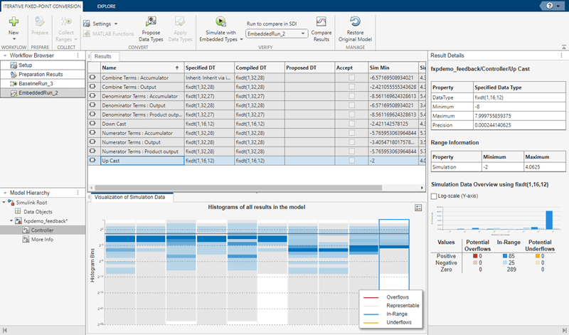
To compare the ideal results stored in BaselineRun with the newly applied fixed-point data types, select EmbeddedRun from the Run to compare in SDI drop down menu. Then click Compare Results to open the Simulation Data Inspector. In the Simulation Data Inspector, select PlantOutput as the signal to compare.
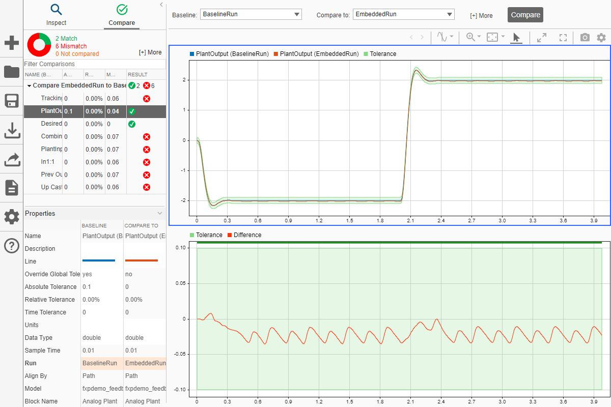
The plot of the plant output signal for EmbeddedRun is within the specified tolerance band. The plant output signal represented by the fixed-point run achieves a steady state, but a small limit cycle is present because of non-optimal A/D design.
If the behavior of the converted system does not meet your requirements or if you want to explore the effect of additional data type selections, you can propose new data types after applying new proposal settings. Continue iterating until you find settings for which the fixed-point behavior of the system is acceptable.
After the conversion process, if you want to restore your model to its state at the start of the conversion process, click Restore Original Model. Any changes made to your model after the preparation stage of conversion are removed.
See Also
Fixed-Point Tool | How Hardware Implementation Settings Affect Data Type Proposals | Iterative Fixed-Point Conversion Using the Fixed-Point Tool