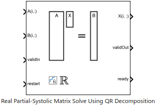
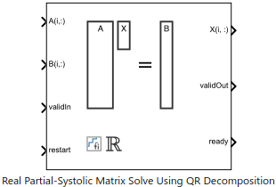
Real Partial-Systolic Matrix Solve Using QR Decomposition

Compute value of x in the equation Ax = B for real-valued matrices using QR decomposition

Since R2020b

• 

×

Libraries:
Fixed-Point Designer HDL Support / Matrices and Linear Algebra / Linear System Solvers

Description

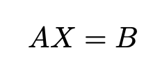
The Real Partial-Systolic Matrix Solve Using QR Decomposition block solves the system of linear equations Ax = B using QR decomposition, where A and B are real-valued matrices. To compute x = A^-1, set B to be the identity matrix.

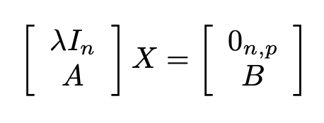
When Regularization parameter is nonzero, the Real Partial-Systolic Matrix Solve Using QR Decomposition block computes the matrix solution of real-valued $$\left[\begin{array}{c}\lambda I_n\\ A\end{array}\right]X=\left[\begin{array}{c}{0}_{n,p}\\ B\end{array}\right]$$ where λ is the regularization parameter, A is an m-by-n matrix, p is the number of columns in B, I_n = eye(n), and 0_n,p = zeros(n,p).

Examples

Implement Hardware-Efficient Real Partial-Systolic Matrix Solve Using QR Decomposition

How to use the Real Partial-Systolic Matrix Solve Using QR Decomposition block.

• Open Script

Implement Hardware-Efficient Real Partial-Systolic Matrix Solve Using QR Decomposition with Diagonal Loading

How to use the Real Partial-Systolic Matrix Solve Using QR Decomposition Block with diagonal loading.

• Open Script

Implement Hardware-Efficient Real Partial-Systolic Matrix Solve Using QR Decomposition with Tikhonov Regularization

Use the Real Partial-Systolic Matrix Solve Using QR Decomposition block to solve the regularized least-squares matrix equation

• Open Script

Algorithms to Determine Fixed-Point Types for Real Least-Squares Matrix Solve AX=B

Derivation of algorithms for determining fixed-point types for real least-squares matrix solve.

• Open Live Script

Determine Fixed-Point Types for Real Least-Squares Matrix Solve AX=B

Use fixed.realQRMatrixSolveFixedpointTypes to determine fixed-point types for computation of the real least-squares matrix equation.

• Open Live Script

Determine Fixed-Point Types for Real Least-Squares Matrix Solve with Tikhonov Regularization

Use the fixed.realQRMatrixSolveFixedpointTypes function to analytically determine fixed-point types for the solution of the real least-squares matrix equation

• Open Live Script

Ports

Input

A(i,:) — Rows of real matrix A

vector

Rows of real matrix A, specified as a vector. A is an m-by-n matrix where m ≥ 2 and m ≥ n. If B is single or double, A must be the same data type as B. If A is a fixed-point data type, A must be signed, use binary-point scaling, and have the same word length as B. Slope-bias representation is not supported for fixed-point data types.

Data Types: single | double | fixed point

B(i,:) — Rows of real matrix B

vector

Rows of real matrix B, specified as a vector. B is an m-by-p matrix where m ≥ 2. If A is single or double, B must be the same data type as A. If B is a fixed-point data type, B must be signed, use binary-point scaling, and have the same word length as A. Slope-bias representation is not supported for fixed-point data types.

Data Types: single | double | fixed point

validIn — Whether inputs are valid

Boolean scalar

Whether inputs are valid, specified as a Boolean scalar. This control signal indicates when the data from the A(i,:) and B(i,:) input ports are valid. When this value is 1 (true) and the value at ready is 1 (true), the block captures the values on the A(i,:) and B(i,:) input ports. When this value is 0 (false), the block ignores the input samples.

After sending a true validIn signal, there may be some delay before ready is set to false. To ensure all data is processed, you must wait until ready is set to false before sending another true validIn signal.

Data Types: Boolean

restart — Whether to clear internal states

Boolean scalar

Whether to clear internal states, specified as a Boolean scalar. When this value is 1 (true), the block stops the current calculation and clears all internal states. When this value is 0 (false) and the validIn value is 1 (true), the block begins a new subframe.

Data Types: Boolean

Output

X(i,:) — Rows of matrix X

scalar | vector

Rows of the matrix X, returned as a scalar or vector.

Data Types: single | double | fixed point

validOut — Whether output data is valid

Boolean scalar

Whether the output data is valid, returned as a Boolean scalar. This control signal indicates when the data at the output port X(i,:) is valid. When this value is 1 (true), the block has successfully computed a row of matrix X. When this value is 0 (false), the output data is not valid.

Data Types: Boolean

ready — Whether block is ready

Boolean scalar

Whether the block is ready, returned as a Boolean scalar. This control signal indicates when the block is ready for new input data. When this value is 1 (true) and the validIn value is 1 (true), the block accepts input data in the next time step. When this value is 0 (false), the block ignores input data in the next time step.

After sending a true validIn signal, there may be some delay before ready is set to false. To ensure all data is processed, you must wait until ready is set to false before sending another true validIn signal.

Data Types: Boolean

Parameters

Number of rows in matrices A and B — Number of rows in matrices A and B

4 (default) | positive integer-valued scalar

Number of rows in input matrices A and B, specified as a positive integer-valued scalar.

Programmatic Use

Block Parameter: m

Type: character vector

Values: positive integer-valued scalar

Default: 4

Number of columns in matrix A — Number of columns in matrix A

4 (default) | positive integer-valued scalar

Number of columns in input matrix A, specified as a positive integer-valued scalar.

Programmatic Use

Block Parameter: n

Type: character vector

Values: positive integer-valued scalar

Default: 4

Number of columns in matrix B — Number of columns in matrix B

1 (default) | positive integer-valued scalar

Number of columns in input matrix B, specified as a positive integer-valued scalar.

Programmatic Use

Block Parameter: p

Type: character vector

Values: positive integer-valued scalar

Default: 1

Regularization parameter — Regularization parameter

0 (default) | real nonnegative scalar

Regularization parameter, specified as a nonnegative scalar. Small, positive values of the regularization parameter can improve the conditioning of the problem and reduce the variance of the estimates. While biased, the reduced variance of the estimate often results in a smaller mean squared error when compared to least-squares estimates.

Programmatic Use

Block Parameter: regularizationParameter

Type: character vector

Values: real nonnegative scalar

Default: 0

Output datatype — Data type of output matrix X

fixdt(1,18,14) (default) | double | single | fixdt(1,16,0) | <data type expression>

Data type of the output matrix X, specified as fixdt(1,18,14), double, single, fixdt(1,16,0), or as a user-specified data type expression. The type can be specified directly, or expressed as a data type object such as Simulink.NumericType.

Programmatic Use

Block Parameter: OutputType

Type: character vector

Values: 'fixdt(1,18,14)' | 'double' | 'single' | 'fixdt(1,16,0)' | '<data type expression>'

Default: 'fixdt(1,18,14)'

Algorithms

Choosing the Implementation Method

Systolic implementations prioritize speed of computations over space constraints, while burst implementations prioritize space constraints at the expense of speed of the operations. The following table illustrates the tradeoffs between the implementations available for matrix decompositions and solving systems of linear equations.

Implementation	Throughput	Latency	Area
Systolic	C	O(n)	O(mn2)
Partial-Systolic	C	O(m)	O(n2)
Partial-Systolic with Forgetting Factor	C	O(n)	O(n2)
Burst	O(n)	O(mn)	O(n)

Where C is a constant proportional to the word length of the data, m is the number of rows in matrix A, and n is the number of columns in matrix A.

For additional considerations in selecting a block for your application, see Choose a Block for HDL-Optimized Fixed-Point Matrix Operations.

AMBA AXI Handshake Process

This block uses the AMBA AXI handshake protocol [1]. The valid/ready handshake process is used to transfer data and control information. This two-way control mechanism allows both the manager and subordinate to control the rate at which information moves between manager and subordinate. A valid signal indicates when data is available. The ready signal indicates that the block can accept the data. Transfer of data occurs only when both the valid and ready signals are high.

Block Timing

The Partial-Systolic Matrix Solve Using QR Decomposition blocks accept and process A and B matrices row by row. After accepting m rows, the block outputs the matrix X as a single vector. The partial-systolic implementation uses a pipelined structure, so the block can accept new matrix inputs before outputting the result of the current matrix.

For example, assume that the input A and B matrices are 3-by-3. Additionally assume that validIn asserts before ready, meaning that the upstream data source is faster than the QR decomposition.

In the figure,

• A1r1 is the first row of the first A matrix and X1 is the matrix X, output as a vector.

• validIn to ready — From a successful row input to the block being ready to accept the next row.

• Last row validIn to validOut — From the last row input to the block starting to output the solution.

The following table provides details of the timing for the Real Partial-Systolic Matrix Solve Using QR Decomposition block. Latency depends on the size of matrix A and the data types of the A and B matrices. In the table:

• m represents the number of rows in matrix A and n is the number of columns in matrix A.

• wl represents the word length of the input data. If the data types of A and B are fixed point or scaled double fi, then wl is given by max(A.WordLength + ~issigned(A), B.WordLength + ~issigned(B)).

Input Data Type	validIn to ready (cycles)	Last Row validIn to validOut (cycles)
Fixed point fi	max(wl + 7, ceil((3.5*n2 + n*(nextpow2(wl) + wl + 8.5) + 6)/m))	(wl + 6)*n + 3.5*n2 + n*(nextpow2(wl) + wl + 9.5) + 9 - n
Scaled double fi	max(wl + 7, ceil((3.5*n2 + n*(wl + 7.5) + 6)/m))	(wl + 6)*n + 3.5*n2 + n*(wl + 7.5) + 9
double	max(60, ceil((3.5*n2 + 6.5*n + 6)/m))	3.5*n2 + 65.5*n + 9
single	max(31, ceil((3.5*n2 + 6.5*n + 6)/m))	3.5*n2 + 36.5*n + 9

Hardware Resource Utilization

This block supports HDL code generation using the Simulink^® HDL Workflow Advisor. For an example, see HDL Code Generation and FPGA Synthesis from Simulink Model (HDL Coder) and Implement Digital Downconverter for FPGA (DSP HDL Toolbox).

In R2022b: The following tables show the post place-and-route resource utilization results and timing summary, respectively.

This example data was generated by synthesizing the block on a Xilinx^® Zynq^® UltraScale™ + RFSoC ZCU111 evaluation board. The synthesis tool was Vivado^® v.2020.2 (win64).

The following parameters were used for synthesis.

• Block parameters:

  • m = 16

  • n = 16

  • p = 1

  • Matrix A dimension: 16-by-16

  • Matrix B dimension: 16-by-1

• Input data type: sfix16_En14

• Target frequency: 300 MHz

Resource	Usage	Available	Utilization (%)
CLB LUTs	110589	425280	26.00
CLB Registers	87850	850560	10.33
DSPs	2	4272	0.05
Block RAM Tile	0	1080	0.00
URAM	0	80	0.00

	Value
Requirement	3.3333 ns
Data Path Delay	3.163 ns
Slack	0.151 ns
Clock Frequency	314.23 MHz

References

[1] "AMBA AXI and ACE Protocol Specification Version E." https://developer.arm.com/documentation/ihi0022/e/AMBA-AXI3-and-AXI4-Protocol-Specification/Single-Interface-Requirements/Basic-read-and-write-transactions/Handshake-process

Extended Capabilities

C/C++ Code Generation

Generate C and C++ code using Simulink® Coder™.

Slope-bias representation is not supported for fixed-point data types.

HDL Code Generation

Generate VHDL, Verilog and SystemVerilog code for FPGA and ASIC designs using HDL Coder™.

HDL Coder™ provides additional configuration options that affect HDL implementation and synthesized logic.

HDL Architecture

This block has one default HDL architecture.

HDL Block Properties

General
ConstrainedOutputPipeline	Number of registers to place at the outputs by moving existing delays within your design. Distributed pipelining does not redistribute these registers. The default is 0. For more details, see ConstrainedOutputPipeline (HDL Coder).
InputPipeline	Number of input pipeline stages to insert in the generated code. Distributed pipelining and constrained output pipelining can move these registers. The default is 0. For more details, see InputPipeline (HDL Coder).
OutputPipeline	Number of output pipeline stages to insert in the generated code. Distributed pipelining and constrained output pipelining can move these registers. The default is 0. For more details, see OutputPipeline (HDL Coder).

Restrictions

Supports fixed-point data types only.

Version History

Introduced in R2020b

R2023a: Smart unrolling for improved resource utilization

This block depends on a partial-systolic QR decomposition block. Since 23a, when you update the diagram, the loop which composes the partial-systolic pipeline in the QR decomposition block is unrolled. This updated internal architecture removes dead operations in simulation and generated code, thus requiring fewer hardware resources. This block simulates with clock and bit-true fidelity with respect to library versions of these blocks in previous releases.