Agency Option-Adjusted Spreads

Often bonds are issued with embedded options, which then makes standard price/yield or spread measures irrelevant. For example, a municipality concerned about the chance that interest rates may fall in the future might issue bonds with a provision that allows the bond to be repaid before the bond’s maturity. This is a call option on the bond and must be incorporated into the valuation of the bond. Option-adjusted spread (OAS), which adjusts a bond spread for the value of the option, is the standard measure for valuing bonds with embedded options. Financial Instruments Toolbox™ software supports computing option-adjusted spreads for bonds with single embedded options using the agency model.

The Securities Industry and Financial Markets Association (SIFMA) has a simplified approach to compute OAS for agency issues (Government Sponsored Entities like Fannie Mae and Freddie Mac) termed “Agency OAS”. In this approach, the bond has only one call date (European call) and uses Black’s model (a variation on Black Scholes, http://en.wikipedia.org/wiki/Black_model) to value the bond option. The price of the bond is computed as follows:

Price_Callable = Price_NonCallable – Price_Option

where

Price_Callable is the price of the callable bond.

Price_NonCallable is the price of the noncallable bond, that is, price of the bond using bndspread.

Price_Option is the price of the option, that is, price of the option using Black’s model.

The Agency OAS is the spread, when used in the previous formula, yields the market price. Financial Instruments Toolbox software supports these functions:

Agency OAS

Agency OAS Functions	Purpose
agencyoas	Compute the OAS of the callable bond using the Agency OAS model.
agencyprice	Price the callable bond OAS using Agency using the OAS model.

Computing the Agency OAS for Bonds

This example shows how to compute Agency OAS for a range of bond prices and the spread of an identically priced noncallable bond.

To compute the Agency OAS using agencyoas, you must provide the zero curve as the input ZeroData. You can specify the zero curve in any intervals and with any compounding method. You can do this using the functions zbtprice and zbtyield. Or, you can use IRDataCurve to construct an IRDataCurve object, and then use the getZeroRates to convert to dates and data for use in the ZeroData input.

After creating the ZeroData input for agencyoas, you can then:

1. Assign parameters for CouponRate, Settle, Maturity, Vol, CallDate, and Price.

2. Compute the option-adjusted spread using agencyoas to derive the OAS output

If you have the Agency OAS for the callable bond, you can use the OAS value as an input to agencyprice to determine the price for a callable bond.

In the following code, the Agency OAS is computed using agencyoas for a range of bond prices and the spread of an identically priced noncallable bond is calculated using bndspread.

%% Data
% Bond data -- Note that there is only 1 call date
Settle = '20-Jan-2010';
Maturity = datetime(2013,12,30);
Coupon = .022;
Vol = .5117;
CallDate = datetime(2010,12,30);
Period = 2;
Basis = 1;
Face = 100;
 
% Zero Curve data
ZeroTime = [.25 .5 1 2 3 4 5 7 10 20 30]';
ZeroDates = daysadd(Settle,360*ZeroTime,1);
ZeroRates = [.0008 .0017 .0045 .0102 .0169 .0224 .0274 .0347 .0414 .0530 .0740]';
ZeroData = [ZeroDates ZeroRates];
CurveCompounding = 2;
CurveBasis = 1;

Price = 94:104;
OAS = agencyoas(ZeroData, Price', Coupon, Settle,Maturity, Vol, CallDate,'Basis',Basis)

OAS = 11×1

  163.4942
  133.7306
  103.8735
   73.7505
   43.1094
   11.5608
  -21.5412
  -57.3869
  -98.5675
 -152.5226
 -239.6462
      ⋮

Spread = bndspread(ZeroData, Price', Coupon, Settle, Maturity)

Spread = 11×1

  168.0988
  139.6637
  111.5726
   83.8177
   56.3915
   29.2869
    2.4967
  -23.9858
  -50.1672
  -76.0538
 -101.6519
      ⋮

plot(OAS,Price)
hold on
plot(Spread,Price,'r')
xlabel('Spread (bp)')
ylabel('Price')
title('AOAS and Spread for an Agency and Equivalent Noncallable Bond')
legend({'Callable Issue','Noncallable Issue'})

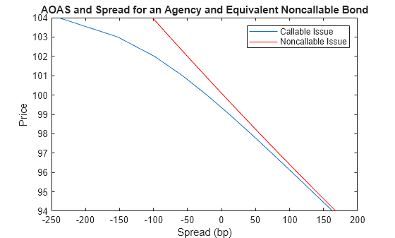
The plot demonstrates as the price increases, the value of the embedded option in the Agency issue increases, and the value of the issue itself does not increase as much as it would for a noncallable bond, illustrating the negative convexity of this issue.