Portfolio Analysis with Turnover Constraints
This example shows how to analyze the characteristics of a portfolio of equities, and then compare them with the efficient frontier. This example seeks to answer the question of how much closer can you get to the efficient frontier by only risking a certain percentage of a portfolio to avoid transaction costs.
Import Data for the Portfolio Holdings
Load information on the current portfolio holdings from a Microsoft® Excel® spreadsheet into a table using the MATLAB® readtable function.
AssetHoldingData = readtable('portfolio.xls');
% Create a normalized current holdings vector that shows the respective
% investments as a percentage of total capital:
W = AssetHoldingData.Value/sum(AssetHoldingData.Value);
Import Market Data for Share Prices
Import the market data from a data source supported by Datafeed Toolbox™ that constitutes three years of closing prices for the stocks listed in the portfolio.
load SharePricesCreate a Portfolio Object
The Portfolio class enables you to use the imported data to create a Portfolio object. The estimateAssetMoments function for the Portfolio object enables you to set up a portfolio given only a historical price or returns series. The estimateAssetMoments function estimates mean and covariance of asset returns from data even if there is missing data.
P = Portfolio('Name', 'Sample Turnover Constraint Portfolio');
P = estimateAssetMoments(P,data,'DataFormat','Prices');

% You can assign text names to each asset in the portfolio.
P = setAssetList(P,AssetHoldingData.Symbol);

% Provide the current holdings.
P = setInitPort(P,W);
Perform Portfolio Optimization with No Turnover Constraint
The Portfolio object can optimize the holdings given any number of constraints. This example demonstrates using a simple, default constraint, that is, long positions only and 100% invested in assets.
P = setDefaultConstraints(P);
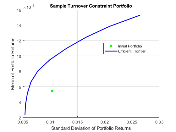
Visualize this efficient frontier with the plotFrontier function.
plotFrontier(P)

Visualize the Transaction Costs and Turnover
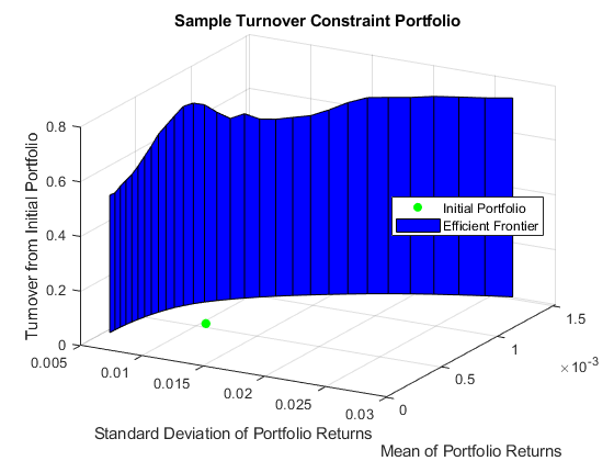
Due to transaction costs, it can be expensive to shift holdings from the current portfolio to a portfolio along this efficient frontier. The following custom plot shows that you must turn over between 50% and 75% of the holdings to get to this frontier.
TurnoverPlot(P)

Perform Portfolio Optimization with a Turnover Constraint
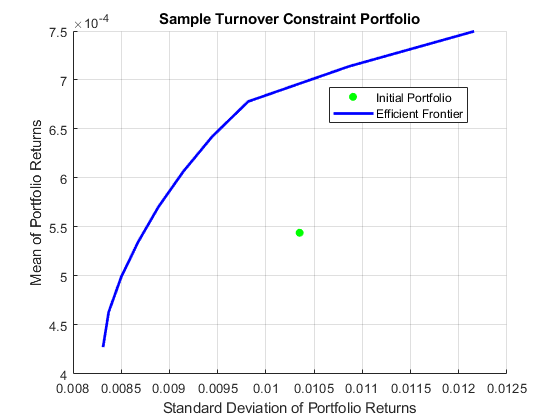
How close can you get to this efficient frontier by only trading some of the portfolio? Assume that you want to trade only a certain percentage of the portfolio to avoid too much turnover in your holdings. This requirement imposes some nonlinear constraints on the problem and gives a problem with multiple local minima. Even so, the Portfolio object solves the problem, and you specify the turnover constraint using the setTurnover function.
P10 = setTurnover(P,0.10);
plotFrontier(P10)

Visualize the Efficient Frontier at Different Turnover Thresholds
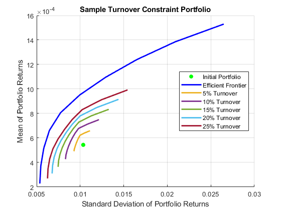
This efficient frontier is much closer to the initial portfolio than the starting efficient frontier without turnover constraints. To visualize this difference, use the custom function TurnoverConstraintPlot to visualize multiple constrained efficient frontiers at different turnover thresholds.
turnovers = 0.05:0.05:0.25;
TurnoverConstraintPlot(P,turnovers)

The Portfolio object is a powerful and efficient tool for performing various portfolio analysis tasks. In addition to turnover constraints, you can also optimize a Portfolio object for transaction costs for buying and selling portfolio assets using the setCosts function.
See Also
Portfolio | setBounds | addGroups | setAssetMoments | estimateAssetMoments | estimateBounds | plotFrontier | estimateFrontierLimits | estimateFrontierByRisk | estimatePortRisk
Topics
- Creating the Portfolio Object
- Working with Portfolio Constraints Using Defaults
- Validate the Portfolio Problem for Portfolio Object
- Estimate Efficient Portfolios for Entire Efficient Frontier for Portfolio Object
- Estimate Efficient Frontiers for Portfolio Object
- Postprocessing Results to Set Up Tradable Portfolios
- Portfolio Optimization with Semicontinuous and Cardinality Constraints
- Black-Litterman Portfolio Optimization Using Financial Toolbox
- Portfolio Optimization Against a Benchmark
- Portfolio Optimization Examples Using Financial Toolbox
- Leverage in Portfolio Optimization with a Risk-Free Asset
- Black-Litterman Portfolio Optimization Using Financial Toolbox
- Portfolio Optimization Using Factor Models
- Portfolio Optimization Using Social Performance Measure
- Diversify Portfolios Using Custom Objective
- Portfolio Object
- Portfolio Optimization Theory
- Portfolio Object Workflow