Adding Constraints to Satisfy UCITS Directive
This example shows how to set up and solve a portfolio optimization problem that satisfies the Undertakings for Collective Investment in Transferable Securities (UCITS) Directive. The UCITS directive is a regulatory requirement of European investment funds. As of 2019, the UCITS asset allocation regulation states that funds can only invest only up to 10% in a single issuer, and that investments in excess of 5% must not exceed 40% of the total portfolio, with some exceptions. This rule is known as the 5/10/40 rule.
Create Portfolio Object
To solve a portfolio problem and add this requirement to the problem, start by creating a Portfolio, PortfolioCVaR, or PortfolioMAD object, depending on the desired risk measure.
% Read table of daily adjusted close prices for 2006 DJI stocks
pricesTT = readtimetable('dowPortfolio.xlsx');
% Compute the returns from the prices
returnsTT = tick2ret(pricesTT);

% Remove the DJI stock from the timetable
assetReturnsTT = returnsTT(:,2:end);
% Compute the asset returns mean and covariance matrix
mu = mean(assetReturnsTT.Variables);
Sigma = cov(assetReturnsTT.Variables);

% Create Portfolio object
p = Portfolio(AssetMean=mu',AssetCovar=Sigma);
To add the 10% upper bound on the maximum that you can invest in any individual asset, use setBounds. In this example, any chosen asset must represent at least 1% of the total portfolio.
% Weights must be either 0 or between 0.01 and 0.1
p = setBounds(p,0.01,0.1,BoundType="conditional");
To set the conditional constraint that limits the aggregate weight that you can invest in assets that exceed 5%, use setConditionalBudget.
% Assets with weights above 5% must not exceed 40% of the total
% portfolio
p = setConditionalBudget(p,0.05,0.4);
Finally, the portfolio weights must sum to one and must have between 15 and 20 active assets.
% Sum of weights must be equal to one
p = setBudget(p,1,1);

% 15-20 active assets
p = setMinMaxNumAssets(p,15,20);
Compute Minimum Variance Portfolio with Tracking Error Penalty
Given some trackingPortfolio weights allocation, find the minimum variance portfolio using estimateCustomObjectivePortfolio with a tracking error penalty that satisfies all the constraints in the previous section.
% Define tracking portfolio as the portfolio of the DJI
trackingPortfolio = returnsTT{:,2:end}\returnsTT{:,1};

% Penalized objective function
penalizedVariance = @(w) w'*Sigma*w + ...
    (w-trackingPortfolio)'*Sigma*(w-trackingPortfolio);

% Penalized variance portfolio
p = setSolverMINLP(p,"OuterApproximation",ExtendedFormulation=true, ...
    ObjectiveScalingFactor=1e4);
w = estimateCustomObjectivePortfolio(p,penalizedVariance);
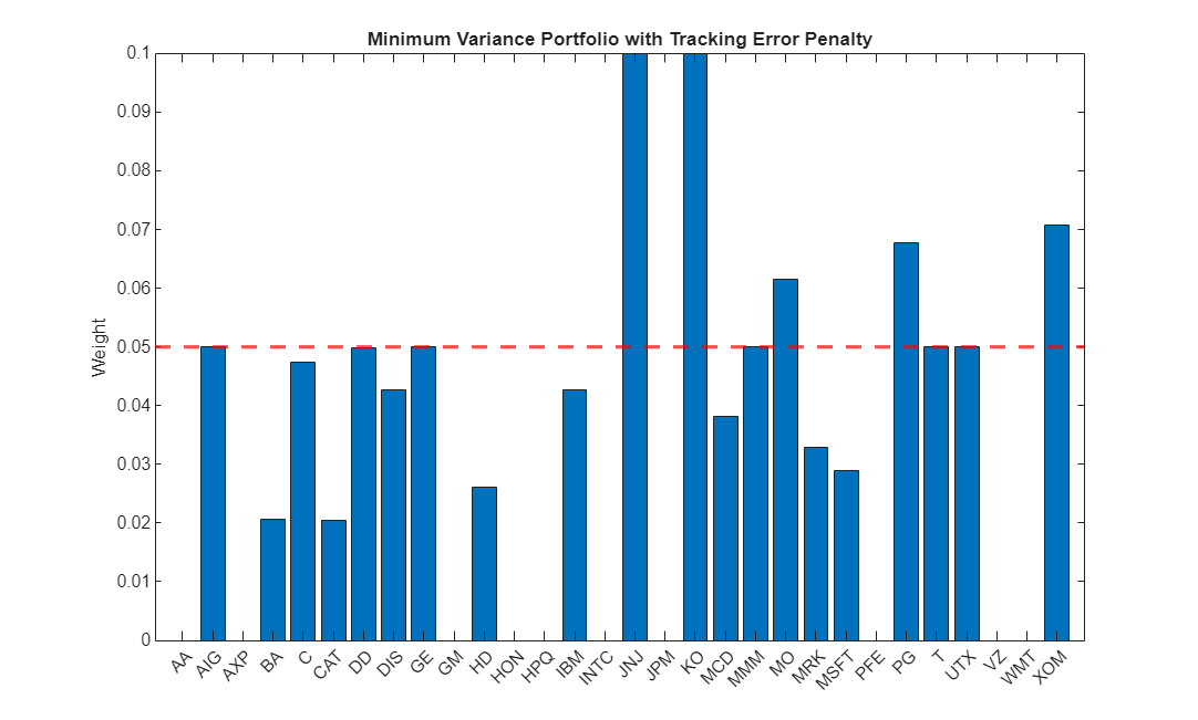
The following bar chart shows the weights distribution of the portfolio.
figure
bar(assetReturnsTT.Properties.VariableNames,w);
hold on
yline(0.05,'r--',LineWidth=2)
title('Minimum Variance Portfolio with Tracking Error Penalty')
ylabel('Weight')

Only five assets are above the 5% conditional threshold and the sum of these assets are less than 40%.
conditionalBudget = sum(w(w > 0.05))
conditionalBudget =
0.4000