Create Regression Models with ARIMA Errors
This topic shows how to represent various regression models with
autoregressive integrated moving average (ARIMA) errors, which are a type of
univariate time series regression
model, as a regARIMA model object. Also, the topic shows
how to interpret the property values of a specified object.
Default Regression Model with ARIMA Errors Specifications
Regression models with ARIMA errors have the following form (in lag operator notation):
where
t = 1,...,T.
yt is the response series.
Xt is row t of X, which is the matrix of concatenated predictor data vectors. That is, Xt is observation t of each predictor series.
c is the regression model intercept.
β is the regression coefficient.
ut is the disturbance series.
εt is the innovations series.
which is the degree p, nonseasonal autoregressive polynomial.
which is the degree ps, seasonal autoregressive polynomial.
which is the degree D, nonseasonal integration polynomial.
which is the degree s, seasonal integration polynomial.
which is the degree q, nonseasonal moving average polynomial.
which is the degree qs, seasonal moving average polynomial.
For simplicity, use the shorthand notation Mdl =
regARIMA(p,D,q) to specify a regression model with
ARIMA(p,D,q) errors,
where p, D, and q are
nonnegative integers. Mdl has the following default
properties.
| Property Name | Property Data Type |
|---|---|
AR | Length p cell vector of
NaNs |
Beta | Empty vector [] of regression
coefficients, corresponding to the predictor series |
D | Nonnegative scalar, corresponding to D |
Distribution | "Gaussian", corresponding to the
distribution of
εt |
Intercept | NaN, corresponding to
c |
MA | Length q cell vector of
NaNs |
P | Number of AR terms plus degree of integration, p + D |
Q | Number of MA terms, q |
SAR | Empty cell vector |
SMA | Empty cell vector |
Variance | NaN, corresponding to the variance of
εt |
Seasonality | 0, corresponding to
s |
If you specify nonseasonal ARIMA errors, then
The properties
DandQare the inputsDandq, respectively.Property
P=p+D, which is the degree of the compound, nonseasonal autoregressive polynomial. In other words,Pis the degree of the product of the nonseasonal autoregressive polynomial, a(L) and the nonseasonal integration polynomial, (1 – L)D.
The values of properties P and
Q indicate how many presample observations the software
requires to initialize the time series.
You can modify the properties of Mdl using dot notation. For
example, Mdl.Variance = 0.5 sets the innovation variance to
0.5.
For maximum flexibility in specifying a regression model with ARIMA errors, use
name-value pair arguments to, for example, set each of the autoregressive parameters
to a value, or specify multiplicative seasonal terms. For example, Mdl =
regARIMA('AR',{0.2 0.1}) defines a regression model with AR(2) errors,
and the coefficients are a1 = 0.2 and
a2 = 0.1.
Specify regARIMA Models Using Name-Value Pair Arguments
You can only specify the nonseasonal autoregressive and moving average polynomial
degrees, and nonseasonal integration degree using the shorthand notation
regARIMA(p,D,q). Some tasks, such as forecasting and
simulation, require you to specify values for parameters. You cannot specify
parameter values using shorthand notation. For maximum flexibility, use name-value
pair arguments to specify regression models with ARIMA errors.
The nonseasonal ARIMA error model might contain the following polynomials:
The degree p autoregressive polynomial a(L) = 1 – a1L – a2L2 –...– apLp. The eigenvalues of a(L) must lie within the unit circle (i.e., a(L) must be a stable polynomial).
The degree q moving average polynomial b(L) = 1 + b1L + b2L2 +...+ bqLq. The eigenvalues of b(L) must lie within the unit circle (i.e., b(L) must be an invertible polynomial).
The degree D nonseasonal integration polynomial is (1 – L)D.
The following table contains the name-value pair arguments that you use to specify the ARIMA error model (i.e., a regression model with ARIMA errors, but without a regression component and intercept):
| (1) |
Name-Value Pair Arguments for Nonseasonal ARIMA Error Models
| Name | Corresponding Model Term(s) in Equation 1 | When to Specify |
|---|---|---|
AR | Nonseasonal AR coefficients: a1, a2,...,ap |
|
ARLags | Lags corresponding to nonzero, nonseasonal AR coefficients |
|
D | Degree of nonseasonal differencing, D |
|
Distribution | Distribution of the innovation process, εt |
|
MA | Nonseasonal MA coefficients: b1, b2,...,bq |
|
MALags | Lags corresponding to nonzero, nonseasonal MA coefficients |
|
Variance | Scalar variance, σ2, of the innovation process, εt | To set equality constraints for
σ2. For
example, for an ARIMA error model with known innovation
variance 0.1, specify |
Use the name-value pair arguments in the following table in conjunction with those in Name-Value Pair Arguments for Nonseasonal ARIMA Error Models to specify the regression components of the regression model with ARIMA errors:
| (2) |
Name-Value Pair Arguments for the Regression Component of the
regARIMA Model
| Name | Corresponding Model Term(s) in Equation 2 | When to Specify |
|---|---|---|
Beta | Regression coefficient values corresponding to the predictor series, β |
|
Intercept | Intercept term for the regression model, c |
|
If the time series has seasonality s, then
The degree ps seasonal autoregressive polynomial is A(L) = 1 – A 1L – A2L2 –...– ApsLps.
The degree qs seasonal moving average polynomial is B(L) 1 + B 1L + B2L2 +...+ BqsLqs.
The degree s seasonal integration polynomial is (1 – Ls).
Use the name-value pair arguments in the following table in conjunction with those in tables Name-Value Pair Arguments for Nonseasonal ARIMA Error Models and Name-Value Pair Arguments for the Regression Component of the regARIMA Model to specify the regression model with multiplicative seasonal ARIMA errors:
| (3) |
Name-Value Pair Arguments for Seasonal ARIMA Models
| Argument | Corresponding Model Term(s) in Equation 3 | When to Specify |
|---|---|---|
SAR | Seasonal AR coefficients: A1, A2,...,Aps |
|
SARLags | Lags corresponding to nonzero seasonal AR coefficients, in the periodicity of the responses |
|
SMA | Seasonal MA coefficients: B1, B2,...,Bqs |
|
SMALags | Lags corresponding to the nonzero seasonal MA coefficients, in the periodicity of the responses |
|
Seasonality | Seasonal periodicity, s |
|
Note
You cannot assign values to the properties P and
Q. For multiplicative ARIMA error models,
regARIMAsetsPequal to p + D + ps + s.regARIMAsetsQequal to q + qs
Specify Linear Regression Models Using Econometric Modeler App
You can specify the predictor variables in the regression component, and the error model lag structure and innovation distribution, using the Econometric Modeler app. The app treats all coefficients as unknown and estimable.
At the command line, open the Econometric Modeler app.
econometricModeler
Alternatively, open the app from the apps gallery (see Econometric Modeler).
In the app, you can see all supported models by selecting a time series variable for the response in the Time Series pane. Then, on the Econometric Modeler tab, in the Models section, click the arrow to display the models gallery.

The Regression Models section contains supported regression
models. To specify a multiple linear regression (MLR) model, select
MLR. To specify regression models with ARMA errors,
select RegARMA.
After you select a model, the app displays the
Type Model Parameters dialog
box, where Type is the model type. This figure shows the
RegARMA Model Parameters dialog box.
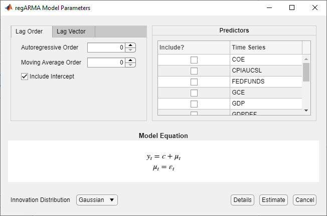
Adjustable parameters depend on the model Type. In
general, adjustable parameters include:
Predictor variables for the linear regression component, listed in the Predictors section.
For regression models with ARMA errors, you must include at least one predictor in the model. To include a predictor, select the corresponding check box in the Include? column.
For MLR models, you can clear all check boxes in the Include? column. In this case, you can specify a constant mean model (intercept-only model) by selecting the Include Intercept check box. Or, you can specify an error-only model by clearing the Include Intercept check box.
The innovation distribution and nonseasonal lags for the error model, for regression models with ARMA errors.
As you adjust parameter values, the equation in the Model
Equation section changes to match your specifications. Adjustable
parameters correspond to input and name-value pair arguments described in the
previous sections and in the regARIMA reference page.
For more details on specifying models using the app, see Fit Models to Data and Specifying Univariate Lag Operator Polynomials Interactively.
What Are Regression Models with Time Series Errors
Regression models with time series errors attempt to explain the mean behavior of a response series (yt, t = 1,...,T) by accounting for linear effects of predictors (Xt) using a multiple linear regression (MLR). However, the errors (ut), called unconditional disturbances, are time series rather than white noise, which is a departure from the linear model assumptions. Unlike the ARIMA model that includes exogenous predictors, regression models with time series errors preserve the sensitivity interpretation of the regression coefficients (β) [3].
These models are particularly useful for econometric data. Use these models to:
Analyze the effects of a new policy on a market indicator (an intervention model).
Forecast population size adjusting for predictor effects, such as expected prevalence of a disease.
Study the behavior of a process adjusting for calendar effects. For example, you can analyze traffic volume by adjusting for the effects of major holidays. For details, see [4].
Estimate the trend by including time (t) in the model.
Forecast total energy consumption accounting for current and past prices of oil and electricity (distributed lag model).
Use these tools in Econometrics Toolbox™ to:
Specify a regression model with ARIMA errors (see
regARIMA).Estimate parameters using a specified model, and response and predictor data (see
estimate).Simulate responses using a model and predictor data (see
simulate).Forecast responses using a model and future predictor data (see
forecast).Infer residuals and estimated unconditional disturbances from a model using the model and predictor data (see
infer).filterinnovations through a model using the model and predictor dataGenerate impulse responses (see
impulse).Compare a regression model with ARIMA errors to an ARIMAX model (see
arima).
A regression model with time series errors has the following form (in lag operator notation):
| (4) |
t = 1,...,T.
yt is the response series.
Xt is row t of X, which is the matrix of concatenated predictor data vectors. That is, Xt is observation t of each predictor series.
c is the regression model intercept.
β is the regression coefficient.
ut is the disturbance series.
εt is the innovations series.
which is the degree p, nonseasonal autoregressive polynomial.
which is the degree ps, seasonal autoregressive polynomial.
which is the degree D, nonseasonal integration polynomial.
which is the degree s, seasonal integration polynomial.
which is the degree q, nonseasonal moving average polynomial.
which is the degree qs, seasonal moving average polynomial.
Following Box and Jenkins methodology, ut is a stationary or unit root nonstationary, regular, linear time series. However, if ut is unit root nonstationary, then you do not have to explicitly difference the series as they recommend in [2]. You can simply specify the seasonal and nonseasonal integration degree using the software.
Another deviation from the Box and Jenkins methodology is that ut does not have a constant term (conditional mean), and therefore its unconditional mean is 0. However, the regression model contains an intercept term, c.
Note
If the unconditional disturbance process is nonstationary (i.e., the nonseasonal or seasonal integration degree is greater than 0), then the regression intercept, c, is not identifiable. For details, see Intercept Identifiability in Regression Models with ARIMA Errors.
The software enforces stability and invertibility of the ARMA process. That is,
where the series {ψt} must be absolutely summable. The conditions for {ψt} to be absolutely summable are:
a(L) and A(L) are stable (i.e., the eigenvalues of a(L) = 0 and A(L) = 0 lie inside the unit circle).
b(L) and B(L) are invertible (i.e., their eigenvalues lie of b(L) = 0 and B(L) = 0 inside the unit circle).
The software uses maximum likelihood for parameter estimation. You can choose either a Gaussian or Student’s t distribution for the innovations, εt.
The software treats predictors as nonstochastic variables for estimation and inference.
What Are Time Series Regression Models?
Time series regression models attempt to explain the current response using the response history (autoregressive dynamics) and the transfer of dynamics from relevant predictors (or otherwise). Theoretical frameworks for potential relationships among variables often permit different representations of the system.
Use time series regression models to analyze time series data, which are measurements that you take at successive time points. For example, use time series regression modeling to:
Examine the linear effects of the current and past unemployment rates and past inflation rates on the current inflation rate.
Forecast GDP growth rates by using an ARIMA model and include the CPI growth rate as a predictor.
Determine how a unit increase in rainfall, amount of fertilizer, and labor affect crop yield.
You can start a time series analysis by building a design matrix (Xt), which can include current and past observations of predictors. You can also complement the regression component with an autoregressive (AR) component to account for the possibility of response (yt) dynamics. For example, include past measurements of inflation rate in the regression component to explain the current inflation rate. AR terms account for dynamics unexplained by the regression component, which is necessarily underspecified in econometric applications. Also, the AR terms absorb residual autocorrelations, simplify innovation models, and generally improve forecast performance. Then, apply ordinary least squares (OLS) to the multiple linear regression (MLR) model:
If a residual analysis suggests classical linear model assumption departures such as that heteroscedasticity or autocorrelation (i.e., nonspherical errors), then:
You can estimate robust HAC (heteroscedasticity and autocorrelation consistent) standard errors (for details, see
hac).If you know the innovation covariance matrix (at least up to a scaling factor), then you can apply generalized least squares (GLS). Given that the innovation covariance matrix is correct, GLS effectively reduces the problem to a linear regression where the residuals have covariance I.
If you do not know the structure of the innovation covariance matrix, but know the nature of the heteroscedasticity and autocorrelation, then you can apply feasible generalized least squares (FGLS). FGLS applies GLS iteratively, but uses the estimated residual covariance matrix. FGLS estimators are efficient under certain conditions. For details, see [1], Chapter 11.
There are time series models that model the dynamics more explicitly than MLR models. These models can account for AR and predictor effects as with MLR models, but have the added benefits of:
Accounting for moving average (MA) effects. Include MA terms to reduce the number of AR lags, effectively reducing the number of observation required to initialize the model.
Easily modeling seasonal effects. In order to model seasonal effects with an MLR model, you have to build an indicator design matrix.
Modeling nonseasonal and seasonal integration for unit root nonstationary processes.
These models also differ from MLR in that they rely on distribution assumptions (i.e., they use maximum likelihood for estimation). Popular types of time series regression models include:
Autoregressive integrated moving average with exogenous predictors (ARIMAX). This is an ARIMA model that linearly includes predictors (exogenous or otherwise). For details, see
arimaor ARIMAX(p,D,q) Model.Regression model with ARIMA time series errors. This is an MLR model where the unconditional disturbance process (ut) is an ARIMA time series. In other words, you explicitly model ut as a linear time series. For details, see
regARIMA.Distributed lag model (DLM). This is an MLR model that includes the effects of predictors that persist over time. In other words, the regression component contains coefficients for contemporaneous and lagged values of predictors. Econometrics Toolbox does not contain functions that model DLMs explicitly, but you can use
regARIMAorfitlmwith an appropriately constructed predictor (design) matrix to analyze a DLM.Transfer function (autoregressive distributed lag) model. This model extends the distributed lag framework in that it includes autoregressive terms (lagged responses). Econometrics Toolbox does not contain functions that model DLMs explicitly, but you can use the
arimafunctionality with an appropriately constructed predictor matrix to analyze an autoregressive DLM.
The choice you make on which model to use depends on your goals for the analysis, and the properties of the data.
References
[1] Greene, William. H. Econometric Analysis. 6th ed. Upper Saddle River, NJ: Prentice Hall, 2008.
[2] Box, George E. P., Gwilym M. Jenkins, and Gregory C. Reinsel. Time Series Analysis: Forecasting and Control. 3rd ed. Englewood Cliffs, NJ: Prentice Hall, 1994.
[3] Hyndman, Rob. J. (2010, October). “The ARIMAX
Model Muddle.” Rob J. Hyndman. Retrieved May 4, 2017
from https://robjhyndman.com/hyndsight/arimax/.
See Also
Apps
Objects
Functions
Topics
- Analyze Time Series Data Using Econometric Modeler
- Specify Default Regression Model with ARIMA Errors
- Modify regARIMA Model Properties
- Create Regression Models with AR Errors
- Create Regression Models with MA Errors
- Create Regression Models with ARMA Errors
- Create Regression Models with SARIMA Errors
- Specify ARIMA Error Model Innovation Distribution
- ARIMAX(p,D,q) Model