forecast
Forecast responses of univariate regression model with ARIMA time series errors
Syntax
Description
[ returns the
Y,YMSE]
= forecast(Mdl,numperiods)numperiods-by-1 numeric vector of consecutive forecasted responses
Y and the corresponding numeric vector of forecast mean square errors
(MSE) YMSE of the fully specified, univariate regression model with
ARIMA time series errors Mdl.
[ also
forecasts a Y,YMSE,U]
= forecast(Mdl,numperiods)numperiods-by-1 numeric vector of unconditional
disturbances U.
[___] = forecast(___,
specifies options using one or more name-value arguments in
addition to any of the input argument combinations in previous syntaxes.
Name=Value)forecast returns the output argument combination for the
corresponding input arguments. For example, forecast(Mdl,10,Y0=y0,X0=Pred0,XF=Pred)
specifies the presample response path y0, and the presample and
forecast sample predictor data Pred0 and Pred,
respectively, to forecast a model with a regression component.
Tbl = forecast(Mdl,numperiods,Presample=Presample,PresampleRegressionDisturbanceVariable=PresampleRegressionDisturbanceVariable)Tbl containing a variable for each of
the paths of response, forecast MSE, and unconditional disturbance series resulting from
forecasting the regression model with ARIMA errors Mdl over a
numperiods forecast horizon. Presample is a
table or timetable containing presample unconditional disturbance data in the variable
specified by PresampleRegressionDisturbanceVariable. Alternatively,
Presample can contain presample error model innovation data in the
variable specified by PresampleInnovationVariable or a combination of
presample response and predictor data in the variables specified by
PresampleResponseVariable and
PresamplePredictorVariables. You can specify either alternative
instead of PresampleRegressionDisturbanceVariable using name-value
syntax; forecast infers presample unconditional disturbance data
from either alternative specification. (since R2023b)
Tbl = forecast(Mdl,numperiods,InSample=InSample,PredictorVariables=PredictorVariables)PredictorVariables in the in-sample table or
timetable of data InSample containing the predictor data for the
model regression component. (since R2023b)
Tbl = forecast(Mdl,numperiods,Presample=Presample,PresampleRegressionDisturbanceVariable=PresampleRegressionDisturbanceVariable,InSample=InSample,PredictorVariables=PredictorVariables)Presample when it is applicable. (since R2023b)
Tbl = forecast(___,Name=Value)
For example,
forecast(Mdl,20,Presample=PSTbl,PresampleResponseVariables="GDP",PresamplePredictorVariables="CPI",InSample=Tbl,PredictorVariables="CPI")
returns a timetable containing variables for the forecasted responses, forecast MSE, and
forecasted unconditional disturbance paths, forecasted 20 periods into the future.
forecast initializes the model by using the presample response
and predictor data in the GDP and CPI variables of
the timetable PSTbl. forecast applies the
predictor data in the PredictorVariables variables of the table or
timetable Tbl to the model regression component.
Examples
Return a vector of responses, forecasted over a 30-period horizon, from the following regression model with ARMA(2,1) errors:
where is Gaussian with variance 0.1.
Specify the model. Simulate responses from the model and two predictor series.
Mdl0 = regARIMA(Intercept=0,AR={0.5 -0.8},MA=-0.5, ...
    Beta=[0.1; -0.2],Variance=0.1);
rng(1,"twister");   % For reproducibility
T = 130;
numperiods = 30;
Pred =  randn(T,2);
y = simulate(Mdl0,T,X=Pred);
Fit the model to the first 100 observations, and reserve the remaining 30 observations to evaluate forecast performance.
Mdl = regARIMA(2,0,1);
estidx = 1:(T-numperiods);  % Estimation sample indices
fhidx = (T-numperiods+1):T; % Forecast horizon
EstMdl = estimate(Mdl,y(estidx),X=Pred(estidx,:));
    Regression with ARMA(2,1) Error Model (Gaussian Distribution):

                   Value      StandardError    TStatistic      PValue
                 _________    _____________    __________    __________

    Intercept    0.0074068      0.012554        0.58999          0.5552
    AR{1}          0.55422      0.087265          6.351      2.1391e-10
    AR{2}         -0.78361      0.080794        -9.6988      3.0499e-22
    MA{1}         -0.46483        0.1394        -3.3345      0.00085446
    Beta(1)       0.092779      0.024497         3.7873      0.00015228
    Beta(2)       -0.17339      0.021143        -8.2008      2.3874e-16
    Variance      0.073721      0.011006         6.6984      2.1066e-11
EstMdl is a new regARIMA model containing the estimates. The estimates are close to their true values.
Use EstMdl to forecast a 30-period horizon.
[yF,yMSE] = forecast(EstMdl,numperiods,Y0=y(estidx), ...
    X0=Pred(estidx,:),XF=Pred(fhidx,:));
yF is a 30-by-1 vector of forecasted responses and yMSE is a 30-by-1 vector of corresponding forecast MSEs. To initialize the model for forecasting, forecast infers required presample unconditional disturbances from the specified presample response and predictor data.
Visually compare the forecasts to the holdout data using a plot.
figure
plot(y,Color=[.7,.7,.7]);
hold on
plot(fhidx,yF,"b",LineWidth=2);
plot(fhidx,yF + 1.96*sqrt(yMSE),"r:",LineWidth=2);
plot(fhidx,yF - 1.96*sqrt(yMSE),"r:",LineWidth=2);
h = gca;
ph = patch([repmat(T-numperiods+1,1,2) repmat(T,1,2)], ...
    [h.YLim fliplr(h.YLim)],[0 0 0 0],"b");
ph.FaceAlpha = 0.1;
legend("Observed","Forecast","95% forecast interval", ...
    Location="best");
title("30-Period Forecasts and 95% Forecast Intervals")
axis tight
hold off
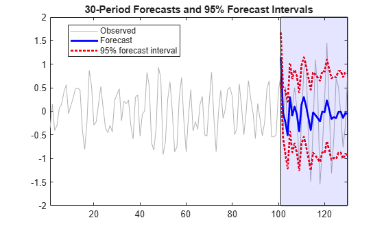
Many observations in the holdout sample fall beyond the 95% forecast intervals. Two reasons for this are:
The predictors are randomly generated in this example.
estimatetreats the predictors as fixed. The 95% forecast intervals based on the estimates fromestimatedo not account for the variability in the predictors.By shear chance, the estimation period seems less volatile than the forecast period.
estimateuses the less volatile estimation period data to estimate the parameters. Therefore, forecast intervals based on the estimates should not cover observations that have an underlying innovations process with larger variability.
Forecast stationary, log GDP using a regression model with ARMA(1,1) errors, including CPI as a predictor.
Fit a regression model with ARMA(1,1) errors by regressing the US gross domestic product (GDP) growth rate onto consumer price index (CPI) quarterly changes. Forecast the model into a 2-year (8-quarter) horizon. Supply a timetable of data and specify the series for the fit.
Load and Transform Data
Load the US macroeconomic data set. Compute the series of GDP quarterly growth rates and CPI quarterly changes.
load Data_USEconModel
DTT = price2ret(DataTimeTable,DataVariables="GDP");
DTT.GDPRate = 100*DTT.GDP;
DTT.CPIDel = diff(DataTimeTable.CPIAUCSL);
T = height(DTT)
T =
248
figure
tiledlayout(2,1)
nexttile
plot(DTT.Time,DTT.GDPRate)
title("GDP Rate")
ylabel("Percent Growth")
nexttile
plot(DTT.Time,DTT.CPIDel)
title("Index")
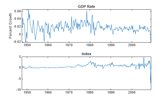
The series appear stationary, albeit heteroscedastic.
Prepare Timetable for Estimation
When you plan to supply a timetable, you must ensure it has all the following characteristics:
The selected response variable is numeric and does not contain any missing values.
The timestamps in the
Timevariable are regular, and they are ascending or descending.
Remove all missing values from the timetable.
DTT = rmmissing(DTT);
T_DTT = height(DTT)
T_DTT =
248
Because each sample time has an observation for all variables, rmmissing does not remove any observations.
Determine whether the sampling timestamps have a regular frequency and are sorted.
areTimestampsRegular = isregular(DTT,"quarters")areTimestampsRegular = logical
0
areTimestampsSorted = issorted(DTT.Time)
areTimestampsSorted = logical
   1
areTimestampsRegular = 0 indicates that the timestamps of DTT are irregular. areTimestampsSorted = 1 indicates that the timestamps are sorted. Macroeconomic series in this example are timestamped at the end of the month. This quality induces an irregularly measured series.
Remedy the time irregularity by shifting all dates to the first day of the quarter.
dt = DTT.Time;
dt = dateshift(dt,"start","quarter");
DTT.Time = dt;
areTimestampsRegular = isregular(DTT,"quarters")
areTimestampsRegular = logical
   1
DTT is regular.
Create Model Template for Estimation
Suppose that a regression model of CPI quarterly changes onto the GDP rate, with ARMA(1,1) errors, is appropriate.
Create a model template for a regression model with ARMA(1,1) errors template. Specify the response variable name.
Mdl = regARIMA(1,0,1);
Mdl.SeriesName = "GDPRate";
Mdl is a partially specified regARIMA object.
Partiton Data
Partition the data set into estimation and forecast samples.
fh = 8;
DTTES = DTT(1:(T_DTT-fh),:);
DTTFS = DTT((T_DTT-fh+1):end,:);
Fit Model to Data
Fit a regression model with ARMA(1,1) errors to the estimation sample. Specify the entire series GDP rate and CPI quarterly changes series, and specify the predictor variable name.
EstMdl = estimate(Mdl,DTTES,PredictorVariables="CPIDel");
    Regression with ARMA(1,1) Error Model (Gaussian Distribution):

                   Value       StandardError    TStatistic      PValue
                 __________    _____________    __________    __________

    Intercept      0.016489      0.0017307        9.5272      1.6152e-21
    AR{1}           0.57835       0.096952        5.9653      2.4415e-09
    MA{1}          -0.15125        0.11658       -1.2974         0.19449
    Beta(1)       0.0025095      0.0014147        1.7738        0.076089
    Variance     0.00011319     7.5405e-06         15.01      6.2792e-51
EstMdl is a fully specified, estimated regARIMA object. By default, estimate backcasts for the required Mdl.P = 1 presample regression model residual and sets the required Mdl.Q = 1 presample error model residual to 0.
Forecast Estimated Model
Forecast the GDP rate over a 8-quarter horizon. Use the estimation sample as a presample for the forecast.
Tbl = forecast(EstMdl,fh,Presample=DTTES,PresampleResponseVariable="GDPRate", ...
    PresamplePredictorVariables="CPIDel",InSample=DTTFS, ...
    PredictorVariables="CPIDel")
Tbl=8×7 timetable
    Time     Interval        GDP         GDPRate      CPIDel    GDPRate_Response    GDPRate_MSE    GDPRate_RegressionInnovation
    _____    ________    ___________    __________    ______    ________________    ___________    ____________________________

    Q2-07       91        0.00018278      0.018278     1.675         0.015765       0.00011319              -0.0049278
    Q3-07       91        0.00016916      0.016916     1.359          0.01705       0.00013383                -0.00285
    Q4-07       94        6.1286e-05     0.0061286     3.355          0.02326       0.00014074              -0.0016483
    Q1-08       91        9.3272e-05     0.0093272      1.93         0.020379       0.00014305             -0.00095329
    Q2-08       91        0.00011103      0.011103     3.367         0.024387       0.00014382             -0.00055134
    Q3-08       92        8.9585e-05     0.0089585     1.641         0.020288       0.00014408             -0.00031887
    Q4-08       92       -0.00016145     -0.016145    -7.098       -0.0015075       0.00014417             -0.00018442
    Q1-09       90       -8.6878e-05    -0.0086878     1.137         0.019236        0.0001442             -0.00010666
Tbl is a 8-by-7 timetable containing the forecasted responses GDPRate_Response and their forecast MSEs GDPRate_MSE, the forecasted unconditional disturbances GDPRate_RegressionInnovation, and all variables in DTTFS.
Plot the forecasts and 95% forecast intervals.
Tbl.Lower = Tbl.GDPRate_Response - 1.96*sqrt(Tbl.GDPRate_MSE);
Tbl.Upper = Tbl.GDPRate_Response + 1.96*sqrt(Tbl.GDPRate_MSE);

figure
h1 = plot(DTT.Time(end-65:end),DTT.GDPRate(end-65:end), ...
    Color=[.7,.7,.7]);
hold on
h2 = plot(Tbl.Time,Tbl.GDPRate_Response,"b",LineWidth=2);
h3 = plot(Tbl.Time,Tbl.Lower,"r:",LineWidth=2);
plot(DTTFS.Time,Tbl.Upper,"r:",LineWidth=2);
ha = gca;
title("GDP Rate Forecasts and 95% Forecast Intervals")
ph = patch([repmat(Tbl.Time(1),1,2) repmat(Tbl.Time(end),1,2)],...
    [ha.YLim fliplr(ha.YLim)],...
    [0 0 0 0],"b");
ph.FaceAlpha = 0.1;
legend([h1 h2 h3],["Observed GDP rate" "Forecasted GDP rate", ...
    "95% forecast interval"],Location="best")
axis tight
hold off

Fit a regression model with ARIMA(1,1,1) errors by regressing the quarterly log US GDP onto the log CPI. Compute MMSE forecasts of the log GDP series using the estimated model. Supply data in timetables.
Load the US macroeconomic data set. Compute the log GDP series.
load Data_USEconModel
DTT = DataTimeTable;
DTT.LogGDP = log(DTT.GDP);
T = height(DTT);
Remedy the time irregularity by shifting all dates to the first day of the quarter.
dt = DTT.Time;
dt = dateshift(dt,"start","quarter");
DTT.Time = dt;
Reserve 2 years (8 quarters) of data at the end of the series to compare against the forecasts.
numperiods = 8;
DTTES = DTT(1:(T-numperiods),:);    % Estimation sample
DTTFS = DTT((T-numperiods+1):T,:);  % Forecast horizon
Suppose that a regression model of the quarterly log GDP on CPI, with ARMA(1,1) errors, is appropriate.
Create a model template for a regression model with ARMA(1,1) errors template. Specify the response variable name.
Mdl = regARIMA(1,1,1);
Mdl.SeriesName = "LogGDP";
The intercept is not identifiable in a regression model with integrated errors. Fix its value before estimation. One way to do this is to estimate the intercept using simple linear regression. Use the estimation sample.
coeff = [ones(T-numperiods,1) DTTES.CPIAUCSL]\DTTES.LogGDP;
Mdl.Intercept = coeff(1);
Consider performing a sensitivity analysis by using a grid of intercepts.
Reserve 2 years (8 quarters) of data at the end of the series to compare against the forecasts.
numperiods = 8;
estidx = 1:(T-numperiods);     % Estimation sample
frstHzn = (T-numperiods+1):T;  % Forecast horizon
Fit a regression model with ARMA(1,1,1) errors to the estimation sample. Specify the predictor variable name.
EstMdl = estimate(Mdl,DTTES,PredictorVariables="CPIAUCSL");
    Regression with ARIMA(1,1,1) Error Model (Gaussian Distribution):

                   Value       StandardError    TStatistic      PValue
                 __________    _____________    __________    ___________

    Intercept        5.8303              0           Inf                0
    AR{1}           0.92869       0.028414        32.684      2.6112e-234
    MA{1}          -0.39063       0.057599       -6.7819       1.1858e-11
    Beta(1)       0.0029335      0.0014645        2.0031         0.045166
    Variance     0.00010668     6.9256e-06        15.403       1.5539e-53
EstMdl is a fully specified, estimated regARIMA object. By default, estimate backcasts for the required Mdl.P = 2 presample regression model residual and sets the required Mdl.Q = 1 presample error model residual to 0.
Infer estimation sample unconditional disturbances to initialize the model for forecasting. Specify the predictor variable name.
Tbl0 = infer(EstMdl,DTTES,PredictorVariables="CPIAUCSL");Forecast the estimated model over an 8-quarter horizon. Use the inferred unconditional disturbances as presample data. Specify the forecast sample predictor data and its variable name, and specify the presample unconditional disturbance variable name.
Tbl = forecast(EstMdl,numperiods,Presample=Tbl0, ...
   PresampleRegressionDisturbanceVariable="LogGDP_RegressionResidual", ...
   InSample=DTTFS,PredictorVariables="CPIAUCSL");
Plot the forecasted log GDP with approximate 95% forecast intervals. Also, separately plot the unconditional disturbances.
Tbl.Lower = Tbl.LogGDP_Response - 1.96*sqrt(Tbl.LogGDP_MSE);
Tbl.Upper = Tbl.LogGDP_Response + 1.96*sqrt(Tbl.LogGDP_MSE);
figure
tiledlayout(2,1)
nexttile
plot(DTT.Time(end-40:end),DTT.LogGDP(end-40:end),Color=[.7,.7,.7])
hold on
h1 = plot(Tbl.Time,[Tbl.Lower Tbl.Upper],"r:",LineWidth=2);
h2 = plot(Tbl.Time,Tbl.LogGDP_Response,"k",LineWidth=2);
h = gca;
ph = patch([repmat(Tbl.Time(1),1,2) repmat(Tbl.Time(end),1,2)], ...
   [h.YLim fliplr(h.YLim)],[0 0 0 0],"b");
ph.FaceAlpha = 0.1;
legend([h1(1) h2],["95% percentile intervals" "MMSE forecast"], ...
    Location="northwest")
axis tight
grid on
title("Log GDP Forecast Over 2-year Horizon")
hold off
nexttile
plot(DTT.Time,[Tbl0.LogGDP_RegressionResidual; Tbl.LogGDP_RegressionInnovation])
hold on
h = gca;
ph = patch([repmat(Tbl.Time(1),1,2) repmat(Tbl.Time(end),1,2)], ...
   [h.YLim fliplr(h.YLim)],[0 0 0 0],"b");
ph.FaceAlpha = 0.1;
axis tight
grid on
title("Unconditional Disturbances")
hold off
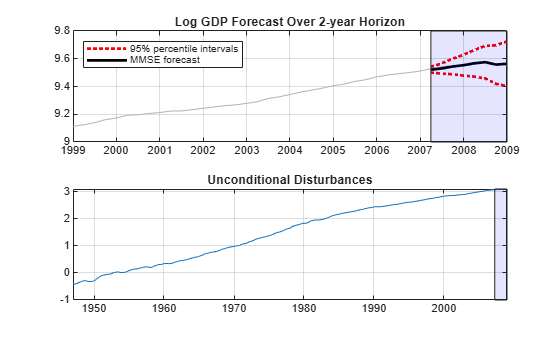
The unconditional disturbances, , are nonstationary, therefore the widths of the forecast intervals grow with time.
Input Arguments
Name-Value Arguments
Output Arguments
More About
Time base partitions for forecasting are two
disjoint, contiguous intervals of the time base; each interval contains time series data for
forecasting a dynamic model. The forecast period (forecast horizon)
is a numperiods length partition at the end of the time base during
which forecast generates forecasts Y from the
dynamic model Mdl. The presample period is the
entire partition occurring before the forecast period. forecast can
require observed responses Y0, regression data X0,
unconditional disturbances U0, or innovations E0
in the presample period to initialize the dynamic model for forecasting. The model structure
determines the types and amounts of required presample observations.
A common practice is to fit a dynamic model to a portion of the data set, then validate
the predictability of the model by comparing its forecasts to observed responses. During
forecasting, the presample period contains the data to which the model is fit, and the
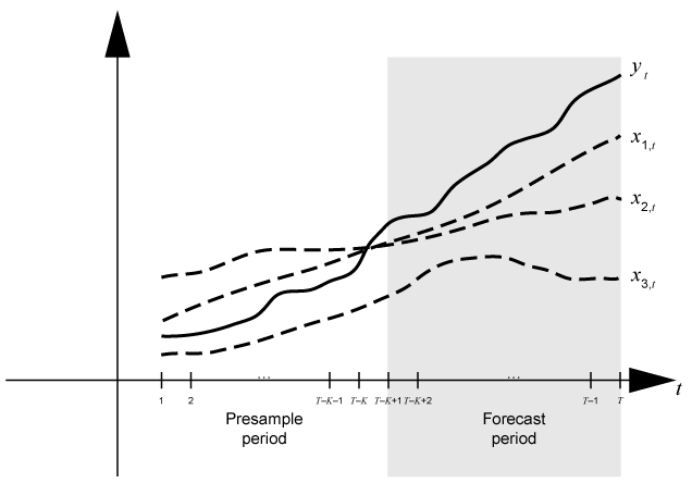
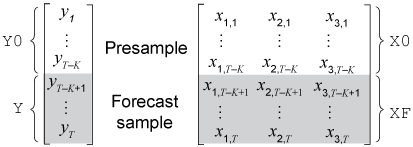
forecast period contains the holdout sample for validation. Suppose that
yt is an observed response series;
x1,t,
x2,t, and
x3,t are observed exogenous
series; and time t = 1,…,T. Consider forecasting
responses from a dynamic model of yt containing a
regression component numperiods = K periods. Suppose
that the dynamic model is fit to the data in the interval [1,T –
K] (for more details, see estimate). This figure shows the time base partitions for forecasting.
For example, to generate forecasts Y from a regression model with
AR(2) errors, forecast requires presample unconditional disturbances
U0 and future predictor data XF.
forecastinfers unconditional disturbances given enough readily available presample responses and predictor data. To initialize an AR(2) error model,Y0= andX0= .To model,
forecastrequires future exogenous dataXF= .
This figure shows the arrays of required observations for the general case, with corresponding input and output arguments.
Algorithms
The
forecastfunction sets the number of sample pathsnumpathsto the maximum number of columns among the specified presample data sets:For input numeric arrays of presample data,
numpathsis the maximum width amongY0,E0, andU0.For an input table or timetable of presample data,
numpathsis the maximum width among the variables representing the presample responsesPresampleResponseVariable, error model innovationsPresampleInnovationVariable, and unconditional disturbancesPresampleRegressionDisturbanceVariable.
All specified presample data sets must have either one column or
numpaths> 1 columns. Otherwise,forecastissues an error. For example, if you supplyY0andE0, andY0has five columns representing five paths, thenE0can have one column or five columns. IfE0has one column,forecastappliesE0to each path.forecastcomputes the forecasted response MSEs by treating the predictor data matrices as nonstochastic and statistically independent of the model innovations. Therefore, the forecast MSEs reflect the variances associated with the unconditional disturbances of the ARIMA error model alone.forecastuses presample response and predictor data to infer presample unconditional disturbances. Therefore, if you specify presample unconditional disturbances,forecastignores any specified presample response and predictor data.
References
[1] Box, George E. P., Gwilym M. Jenkins, and Gregory C. Reinsel. Time Series Analysis: Forecasting and Control. 3rd ed. Englewood Cliffs, NJ: Prentice Hall, 1994.
[2] Davidson, R., and J. G. MacKinnon. Econometric Theory and Methods. Oxford, UK: Oxford University Press, 2004.
[3] Enders, Walter. Applied Econometric Time Series. Hoboken, NJ: John Wiley & Sons, Inc., 1995.
[4] Hamilton, James D. Time Series Analysis. Princeton, NJ: Princeton University Press, 1994.
[5] Pankratz, A. Forecasting with Dynamic Regression Models. John Wiley & Sons, Inc., 1991.
[6] Tsay, R. S. Analysis of Financial Time Series. 2nd ed. Hoboken, NJ: John Wiley & Sons, Inc., 2005.