chowtest
Chow test for structural change
Syntax
Description
h = chowtest(X,y,bp)y =
Xβ + ε at specified
break points. y is a vector of response data and
X is a matrix of predictor data. Each element of
bp results in a separate test.
StatTbl = chowtest(Tbl,bp)StatTbl containing variables for the test
results, statistics, and settings from conducting Chow tests on the variables of the
table or timetable Tbl. Each row of
StatTbl contains the results of the corresponding
test.
The response variable in the regression is the last table variable, and all other
variables are the predictor variables. To select a different response variable for
the regression, use the ResponseVariable name-value argument.
To select different predictor variables, use the PredictorNames
name-value argument.
___ = chowtest(___,
specifies options using one or more name-value arguments in
addition to any of the input argument combinations in previous syntaxes.
Name=Value)chowtest returns the output argument combination for the
corresponding input arguments.
In addition to bp, some options control the number of tests
to conduct. For example,
chowtest(Tbl,ResponseVariable="GDP",Test=["breakpoint"
"forecast"],Intercept=false) conducts two tests for the presence of a
structural break in the coefficients of the regression model of
GDP on all other variables of the table
Tbl without an intercept term. The first test assesses
coefficient equality constraints directly, and the second test assesses forecast
performance.
Examples
Conduct Chow tests to assess whether there are structural changes in the equation for food demand around World War II. Input the predictor series as a matrix and input the response series as a vector.
Load the US food consumption data set Data_Consumption.mat, which contains annual measurements from 1927 through 1962 with missing data due to the war in the matrix Data.
load Data_ConsumptionSuppose that you want to develop a model for consumption as determined by food prices and disposable income, and assess its stability through the economic shock through the war.
Plot the series.
P = Data(:,1); % Food price index I = Data(:,2); % Disposable income index Q = Data(:,3); % Food consumption index figure; plot(dates,[P I Q]) axis tight grid on xlabel("Year") ylabel("Index") legend(["Price" "Income" "Consumption"],Location="southeast")
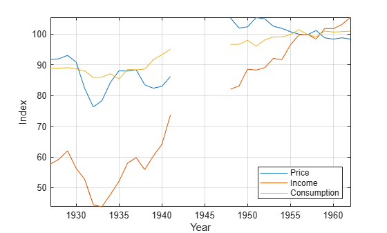
Measurements are missing from 1942 through 1947, which correspond to World War II.
Stabilize each series by applying the log transformation.
LP = log(P); LI = log(I); LQ = log(Q);
Assume that log consumption is a linear function of the logs of food price and income.
is a Gaussian random variable with mean 0 and standard deviation .
Identify the indices before World War II. Plot log consumption with respect to the logs of food price and income.
preWarIdx = (dates <= 1941); figure scatter3(LP(preWarIdx),LI(preWarIdx),LQ(preWarIdx),[],"ro"); hold on scatter3(LP(~preWarIdx),LI(~preWarIdx),LQ(~preWarIdx),[],"b*"); legend(["Pre-war observations" "Post-war observations"], ... Location="best") xlabel("Log Price") ylabel("Log Income") zlabel("Log Consumption") % Obtain better view h = gca; h.CameraPosition = [4.3 -12.2 5.3];
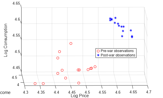
Data relationships appear to be affected by the war.
Conduct two break point Chow tests at 5% level of significance. For the first test, set the break point at 1941. Set the break point of the other test at 1948.
bp = find(preWarIdx,1,"last");
X = [LP LI];
y = LQ;
h1941 = chowtest(X,y,bp) h1941 = logical
1
h1948 = chowtest(X,y,bp + 1)
h1948 = logical
0
h1941 = 1 indicates that there is enough evidence to reject the null hypothesis that the coefficients are stable when the break points occur before the war. However, h1948 = 0 indicates that there is not enough evidence to reject coefficient stability if the break point is after the war. This result suggests that the data at 1948 is influential.
Alternatively, you can supply a vector of break points to conduct three Chow tests.
h = chowtest(X,y,[bp bp+1]);
RESULTS SUMMARY *************** Test 1 Sample size: 30 Breakpoint: 15 Test type: breakpoint Coefficients tested: All Statistic: 5.5400 Critical value: 3.0088 P value: 0.0049 Significance level: 0.0500 Decision: Reject coefficient stability *************** Test 2 Sample size: 30 Breakpoint: 16 Test type: breakpoint Coefficients tested: All Statistic: 1.2942 Critical value: 3.0088 P value: 0.2992 Significance level: 0.0500 Decision: Fail to reject coefficient stability
By default, chowtest displays a summary of the test results for each test when you conduct more than one test.
Load the US food consumption data set Data_Consumption.mat. Consider a model for log food consumption as determined by log food prices and log disposable income.
load Data_Consumption
X = log(Data(:,1:2));
y = log(Data(:,3));Conduct two break point Chow tests at 5% level of significance. For the first test, set the break point at 1941. Set the break point of the other test at 1948. Return the test decision, -Value, test statistic, and test critical value.
bp = find(dates <= 1941,1,"last");
[h,pValue,stat,cValue] = chowtest(X,y,bp)h = logical
1
pValue = 0.0049
stat = 5.5400
cValue = 3.0088
pValue < 0.01, which suggests that the evidence to reject the null hypothesis that all coefficients in the regression models, determined by the break point at 1941, are equal.
Conduct Chow tests to assess whether there are structural changes in the equation for food demand around World War II, where the time series are variables in a table.
Load the US food consumption data set Data_Consumption.mat, which contains annual measurements from 1927 through 1962 with missing data due to the war in the table DataTable. Convert the table to a timetable, and remove rows containing missing values.
load Data_Consumption
dates = datetime(dates,12,31);
TT = table2timetable(DataTable,RowTimes=dates);
TT.Row = [];
TT = rmmissing(TT);Apply the log transform to all variables in the table.
LogTT = varfun(@log,TT); LogTT.Properties.VariableNames
ans = 1×3 cell
{'log_P'} {'log_I'} {'log_Q'}
Conduct two break point Chow tests at 5% level of significance. For the first test, set the break point at the end of 1941. Set the break point of the other test at the end of 1948.
bp1941 = find(LogTT.Time >= datetime(1941,12,31),1); bp1948 = find(LogTT.Time >= datetime(1948,12,31),1); bp = [bp1941 bp1948]; StatTbl = chowtest(LogTT,bp)
RESULTS SUMMARY

***************
Test 1

Sample size: 30
Breakpoint: 15

Test type: breakpoint
Coefficients tested: All

Statistic: 5.5400
Critical value: 3.0088

P value: 0.0049
Significance level: 0.0500

Decision: Reject coefficient stability

***************
Test 2

Sample size: 30
Breakpoint: 16

Test type: breakpoint
Coefficients tested: All

Statistic: 1.2942
Critical value: 3.0088

P value: 0.2992
Significance level: 0.0500

Decision: Fail to reject coefficient stability
StatTbl=2×8 table
                h       pValue       stat     cValue    Break Point    Alpha    Intercept         Test
              _____    _________    ______    ______    ___________    _____    _________    ______________

    Test 1    true     0.0049125      5.54    3.0088        15         0.05       true       {'breakpoint'}
    Test 2    false      0.29918    1.2942    3.0088        16         0.05       true       {'breakpoint'}
StatTbl contains the decision statistics and options for each test (row).
By default, chowtest selects the last table variable as the response, and selects all other variables as predictors. You can select a different variable by using the ResponseVariable name-value argument. You can choose a different set of predictor variables by using the PredictorVariables name-value argument.
Apply the Chow test to assess the stability of an explanatory model of US real gross national product (RGNP) using the end of World War II as a break point.
Load the Nelson-Plosser data set Data_NelsonPlosser.mat, which contains the table of data DataTable.
load Data_NelsonPlosserThe time series in the data set contain annual, macroeconomic measurements from 1860 to 1970. For more details, a list of variables, and descriptions, enter Description in the command line.
Convert the table to a timetable. Focus the sample to measurements from the end of 1915 through the end of 1970.
dates = datetime(dates,12,31);
span = isbetween(dates,datetime(1915,12,31),datetime(1970,12,31),"closed");
TT = table2timetable(DataTable,RowTimes=dates);
TT.Dates = [];
TT = TT(span,:);
Consider a predictive model of the US RGNP GNPR given measurements of the industrial production index IPI, total employment E, and real wages WR.
Plot the series in the model.
prednames = ["IPI" "E" "WR"];

tiledlayout(2,2)
for j = ["GNPR" prednames]
    nexttile
    plot(TT.Time,TT{:,j})
    ylabel(j)
end

To address exponential growth, apply the log transform to the series.
LogTT = varfun(@log,TT);
LogTT is a timetable containing the transformed variables in TT, but with names prepended with log_.
Select the index corresponding to the end of World War II, September 2, 1945.
bp = find(LogTT.Time > datetime(1945,9,2),1);
Assume that an appropriate multiple regression model to describe real GNP is
Conduct a break point test to assess whether all regression coefficients are stable. Use the end of WWII as a break point. Print a test summary to the command line.
lprednames = "log_" + prednames;
StatTbl = chowtest(LogTT,bp,ResponseVariable="log_GNPR", ...
    PredictorVariables=lprednames,Display="summary")
RESULTS SUMMARY

***************
Test 1

Sample size: 56
Breakpoint: 31

Test type: breakpoint
Coefficients tested: All

Statistic: 4.0978
Critical value: 2.5652

P value: 0.0062
Significance level: 0.0500

Decision: Reject coefficient stability
StatTbl=1×8 table
                h       pValue       stat     cValue    Break Point    Alpha    Intercept         Test
              _____    _________    ______    ______    ___________    _____    _________    ______________

    Test 1    true     0.0061633    4.0978    2.5652        31         0.05       true       {'breakpoint'}
StatTbl contains decision statistics and test options for the test. StatTbl.h = 1 and StatTbl.pValue < 0.01 indicate string evidence to reject the null hypothesis that the regression coefficients before and after WWII are equivalent.
Conduct a Chow test to assess the stability of a subset of regression coefficients. This example expands on Conduct Chow Test for Structural Change.
Load the US food consumption data set. Convert the table to a timetable, and remove rows containing missing values.
load Data_Consumption.mat
dates = datetime(dates,12,31);
TT = table2timetable(DataTable,RowTimes=dates);
TT.Row = [];
TT = rmmissing(TT);
Apply the log transformation to each series.
LogTT = varfun(@log,DataTable);
Identify the indices before World War II.
preWarIdx = dates <= datetime(1941,12,31);
Consider two regression models: one is log consumption onto log food price, and the other is log consumption onto log income. Plot scatter plots and regression lines for both models.
figure
plot(LogTT.log_P(preWarIdx),LogTT.log_Q(preWarIdx),"bo", ...
    LogTT.log_P(~preWarIdx),LogTT.log_Q(~preWarIdx),"r*");
axis tight
grid on
lsline
xlabel("Log Price")
ylabel("Log Consumption")
legend("Pre-war observations","Post-war observations")
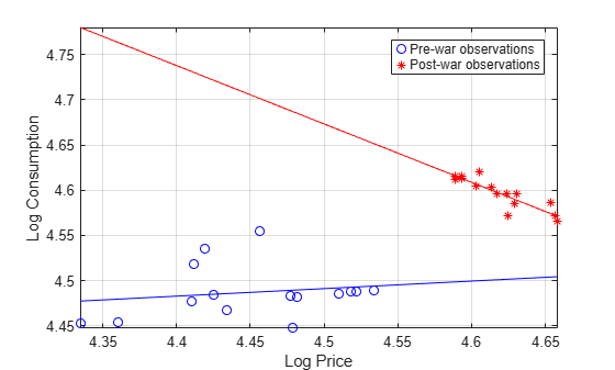
figure
plot(LogTT.log_I(preWarIdx),LogTT.log_Q(preWarIdx),"bo", ...
    LogTT.log_I(~preWarIdx),LogTT.log_Q(~preWarIdx),"r*");
axis tight
grid on
lsline
xlabel("Log Income")
ylabel("Log Consumption")
legend("Pre-war observations","Post-war observations", ...
    Location="northwest")

A clear break in food price elasticity exists between subsamples before and after the war. However, income elasticity does not appear to have such a break.
Conduct two Chow tests to determine whether there is statistical evidence to reject model continuity for both regression models. Because there are more observations in the complementary subsample than coefficients, conduct a break point test. Consider the elasticities in the test only. That is, specify false for the intercept (first coefficient) and true for elasticity (second coefficient).
bp = find(preWarIdx,1,"last"); % Index for 1941
chowtest(LogTT,bp,Coeffs=[false true],Display="summary", ...
    ResponseVariable="log_Q",PredictorVariables="log_P");
RESULTS SUMMARY

***************
Test 1

Sample size: 30
Breakpoint: 15

Test type: breakpoint
Coefficients tested: 0  1

Statistic: 7.3947
Critical value: 4.2252

P value: 0.0115
Significance level: 0.0500

Decision: Reject coefficient stability
chowtest(LogTT,bp,Coeffs=[false true],Display="summary", ...
    ResponseVariable="log_Q",PredictorVariables="log_I");
RESULTS SUMMARY

***************
Test 1

Sample size: 30
Breakpoint: 15

Test type: breakpoint
Coefficients tested: 0  1

Statistic: 0.1289
Critical value: 4.2252

P value: 0.7225
Significance level: 0.0500

Decision: Fail to reject coefficient stability
The first test rejects the null hypothesis that price elasticities are equivalent across subsamples at 5% level of significance. The second test fails to reject the null hypothesis that income elasticities are equivalent across subsamples.
Consider a regression model of log consumption onto the logs of price and income. Conduct two break point tests: one that compares price elasticity across subsamples only, and another that compares income elasticity only.
Coeffs = [false true false;
          false false true];
chowtest(LogTT,bp,Coeffs=Coeffs,Display="summary", ...
    ResponseVariable="log_Q",PredictorVariables=["log_P" "log_I"]);
RESULTS SUMMARY *************** Test 1 Sample size: 30 Breakpoint: 15 Test type: breakpoint Coefficients tested: 0 1 0 Statistic: 0.0001 Critical value: 4.2597 P value: 0.9920 Significance level: 0.0500 Decision: Fail to reject coefficient stability *************** Test 2 Sample size: 30 Breakpoint: 15 Test type: breakpoint Coefficients tested: 0 0 1 Statistic: 2.8151 Critical value: 4.2597 P value: 0.1064 Significance level: 0.0500 Decision: Fail to reject coefficient stability
For both tests, there is not enough evidence to reject model stability at 5% level.
Simulate data for a linear model including a structural break in the intercept and one of the predictor coefficients. Then, choose specific coefficients to test for equality across a break point using the Chow test. Adjust parameters to assess the sensitivity of the Chow test.
Specify four predictors, 50 observations, and a break point at period 44 for the simulated linear model.
numPreds = 4;
numObs = 50;
bp = 44;
rng(1); % For reproducibility
Form the predictor data by specifying means for the predictors, and then adding random, standard Gaussian noise to each of the means.
mu = [0 1 2 3];
X = repmat(mu,numObs,1) + randn(numObs,numPreds);
Include a column of ones to the predictor data.
X = [ones(numObs,1) X];
Specify the true values of the regression coefficients and that the intercept and the coefficient of the second predictor jump by 10%.
beta1 = [1 2 3 4 5]';                                % Initial subsample coefficients
beta2 = beta1 + [beta1(1)*0.1 0 beta1(3)*0.1 0 0 ]'; % Complementary subsample coefficients
X1 = X(1:bp,:);                                      % Initial subsample predictors
X2 = X(bp+1:end,:);                                  % Complementary subsample predictors
Specify a 2-by-5 logical matrix that indicates to test first the intercept and second regression coefficient, and then test all other coefficients.
test1 = [true false true false false];
Coeffs = [test1; ~test1]
Coeffs = 2×5 logical array

   1   0   1   0   0
   0   1   0   1   1
The null hypothesis for the first test (Coeffs(1,:)) is equality of the intercepts and the coefficients of the second predictor across subsamples. The null hypothesis for the second test (Coeffs(2,:)) is equality of the first, third, and fourth predictors across subsamples.
Simulate data for the linear model
Create innov as a vector of random Gaussian variates with mean zero and standard deviation 0.2.
sigma = 0.2;
innov = sigma*randn(numObs,1);
y = [X1 zeros(bp,size(X2,2)); ...
    zeros(numObs-bp,size(X1,2)) X2]*[beta1; beta2]+innov;
Conduct the two break point tests indicated in Coeffs. Because there is an intercept in the predictor matrix X already, specify to suppress its inclusion in the linear model that chowtest fits.
chowtest(X,y,bp,Intercept=false,Coeffs=Coeffs, ...
    Display="summary");
RESULTS SUMMARY

***************
Test 1

Sample size: 50
Breakpoint: 44

Test type: breakpoint
Coefficients tested: 1  0  1  0  0

Statistic: 5.7102
Critical value: 3.2317

P value: 0.0066
Significance level: 0.0500

Decision: Reject coefficient stability

***************
Test 2

Sample size: 50
Breakpoint: 44

Test type: breakpoint
Coefficients tested: 0  1  0  1  1

Statistic: 0.2497
Critical value: 2.8387

P value: 0.8611
Significance level: 0.0500

Decision: Fail to reject coefficient stability
At the default significance level:
The Chow test correctly rejects the null hypothesis that no structural breaks exist at period
bpfor the intercept and the second coefficient.The Chow test correctly failed to reject the null hypothesis for the other coefficients.
Compare the break point test results to the results of the forecast test.
chowtest(X,y,bp,Intercept=false,Coeffs=Coeffs, ...
    Test="forecast",Display="summary");
RESULTS SUMMARY

***************
Test 1

Sample size: 50
Breakpoint: 44

Test type: forecast
Coefficients tested: 1  0  1  0  0

Statistic: 3.7637
Critical value: 2.8451

P value: 0.0182
Significance level: 0.0500

Decision: Reject coefficient stability

***************
Test 2

Sample size: 50
Breakpoint: 44

Test type: forecast
Coefficients tested: 0  1  0  1  1

Statistic: 0.2135
Critical value: 2.6123

P value: 0.9293
Significance level: 0.0500

Decision: Fail to reject coefficient stability
In this case, the inferences from the tests are equivalent to those for the break point test.
Input Arguments
Name-Value Arguments
Output Arguments
More About
Tips
Chow tests assume continuity of the innovations variance across structural changes. Heteroscedasticity can distort the size and power of the test. Therefore, verify the innovations-variance-continuity assumption holds before using the test results for inference.
If both subsamples contain more than
numCoeffsobservations, you can conduct a forecast test instead of a break point test (seeTest). However, the forecast test might have lower power relative to the break point test [1]. Nevertheless, Wilson (1978) suggests conducting the forecast test in the presence of unknown specification errors [4].You can apply the forecast test to cases where both subsamples have size greater than
numCoeffs, where you would typically apply a breakpoint test. In such cases, the forecast test might have significantly reduced power relative to a break point test [1]. Nevertheless, Wilson (1978) suggests use of the forecast test in the presence of unknown specification errors [4].The forecast test is based on the unbiased predictions, with zero mean error, that result from stable coefficients. However, zero mean forecast error does not, in general, guarantee coefficient stability. Therefore, forecast tests are most effective in checking for structural breaks, rather than model continuity [3].
To obtain diagnostic statistics for each subsample, such as regression coefficient estimates, their standard errors, error sums of squares, and so on, pass the appropriate data to
fitlm. For details on working withLinearModelmodel objects, see Multiple Linear Regression.
References
[1] Chow, G. C. "Tests of Equality Between Sets of Coefficients in Two Linear Regressions." Econometrica. Vol. 28, 1960, pp. 591–605.
[2] Fisher, F. M. "Tests of Equality Between Sets of Coefficients in Two Linear Regressions: An Expository Note." Econometrica. Vol. 38, 1970, pp. 361–66.
[3] Rea, J. D. "Indeterminacy of the Chow Test When the Number of Observations is Insufficient." Econometrica. Vol. 46, 1978, p. 229.
[4] Wilson, A. L. "When is the Chow Test UMP?" The American Statistician. Vol. 32, 1978, pp. 66–68.
Version History
Introduced in R2015bSee Also
fitlm | LinearModel | cusumtest | recreg