Create Autoregressive Integrated Moving Average Models
These examples show how to create various autoregressive integrated moving
average (ARIMA) models by using the arima function.
Default ARIMA Model
This example shows how to use the shorthand arima(p,D,q) syntax to specify the default ARIMA(p, D, q) model,
where is a differenced time series. You can write this model in condensed form using lag operator notation:
By default, all parameters in the created model object have unknown values, and the innovation distribution is Gaussian with constant variance.
Specify the default ARIMA(1,1,1) model:
Mdl = arima(1,1,1)
Mdl =
  arima with properties:

     Description: "ARIMA(1,1,1) Model (Gaussian Distribution)"
      SeriesName: "Y"
    Distribution: Name = "Gaussian"
               P: 2
               D: 1
               Q: 1
        Constant: NaN
              AR: {NaN} at lag [1]
             SAR: {}
              MA: {NaN} at lag [1]
             SMA: {}
     Seasonality: 0
            Beta: [1×0]
        Variance: NaN
The output shows that the created model object, Mdl, has NaN values for all model parameters: the constant term, the AR and MA coefficients, and the variance. You can modify the created model using dot notation, or input it (along with data) to estimate.
The property P has value 2 (p + D). This is the number of presample observations needed to initialize the AR model.
ARIMA Model with Known Parameter Values
This example shows how to specify an ARIMA(p, D, q) model with known parameter values. You can use such a fully specified model as an input to simulate or forecast.
Specify the ARIMA(2,1,1) model
where the innovation distribution is Student's t with 10 degrees of freedom, and constant variance 0.15.
tdist = struct('Name','t','DoF',10);
Mdl = arima('Constant',0.4,'AR',{0.8,-0.3},'MA',0.5,...
    'D',1,'Distribution',tdist,'Variance',0.15)
Mdl =
  arima with properties:

     Description: "ARIMA(2,1,1) Model (t Distribution)"
      SeriesName: "Y"
    Distribution: Name = "t", DoF = 10
               P: 3
               D: 1
               Q: 1
        Constant: 0.4
              AR: {0.8 -0.3} at lags [1 2]
             SAR: {}
              MA: {0.5} at lag [1]
             SMA: {}
     Seasonality: 0
            Beta: [1×0]
        Variance: 0.15
The name-value pair argument D specifies the degree of nonseasonal integration (D).
All parameter values are specified, that is, no object property is NaN-valued.
Specify ARIMA Model Using Econometric Modeler App
In the Econometric Modeler app, you can specify the lag structure, presence of a constant, and innovation distribution of an ARIMA(p,D,q) model by following these steps. All specified coefficients are unknown but estimable parameters.
At the command line, open the Econometric Modeler app.
econometricModeler
Alternatively, open the app from the apps gallery (see Econometric Modeler).
In the Time Series pane, select the response time series to which the model will be fit.
On the Econometric Modeler tab, in the Models section, click ARIMA. To create ARIMAX models, see Create ARIMA Models That Include Exogenous Covariates.
The ARIMA Model Parameters dialog box appears.
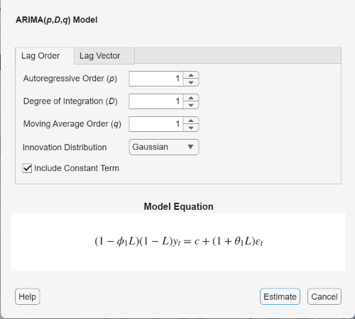
Specify the lag structure. To specify an ARIMA(p,D,q) model that includes all AR lags from 1 through p and all MA lags from 1 through q, use the Lag Order tab. For the flexibility to specify the inclusion of particular lags, use the Lag Vector tab. For more details, see Specifying Univariate Lag Operator Polynomials Interactively. Regardless of the tab you use, you can verify the model form by inspecting the equation in the Model Equation section.
For example:
To specify an ARIMA(3,1,2) model that includes a constant, includes all consecutive AR and MA lags from 1 through their respective orders, and has a Gaussian innovation distribution:
Set Degree of Integration to
1.Set Autoregressive Order to
3.Set Moving Average Order to
2.
To specify an ARIMA(3,1,2) model that includes all AR and MA lags from 1 through their respective orders, has a Gaussian distribution, but does not include a constant:
Set Degree of Integration to
1.Set Autoregressive Order to
3.Set Moving Average Order to
2.Clear the Include Constant Term check box.
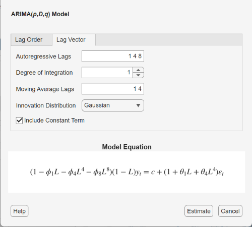
To specify an ARIMA(8,1,4) model containing nonconsecutive lags
where εt is a series of IID Gaussian innovations:
Click the Lag Vector tab.
Set Degree of Integration to
1.Set Autoregressive Lags to
1 4 8.Set Moving Average Lags to
1 4.Clear the Include Constant Term check box.
To specify an ARIMA(3,1,2) model that includes all consecutive AR and MA lags through their respective orders and a constant term, and has t-distribution innovations:
Set Degree of Integration to
1.Set Autoregressive Order to
3.Set Moving Average Order to
2.Click the Innovation Distribution button, then select
t.
The degrees of freedom parameter of the t distribution is an unknown but estimable parameter.
After you specify a model, click Estimate to estimate all unknown parameters in the model.
What Are ARIMA Models?
The autoregressive integrated moving average (ARIMA) process generates nonstationary series that are integrated of order D, denoted I(D). A nonstationary I(D) process is one that can be made stationary by taking D differences. Such processes are often called difference-stationary or unit root processes.
A series that you can model as a stationary ARMA(p,q) process after being differenced D times is denoted by ARIMA(p,D,q). The form of the ARIMA(p,D,q) model in Econometrics Toolbox™ is
| (1) |
In lag operator notation, . You can write the ARIMA(p,D,q) model as
| (2) |
The signs of the coefficients in the AR lag operator polynomial, , are opposite to the right side of Equation 1. When specifying and interpreting AR coefficients in Econometrics Toolbox, use the form in Equation 1.
Note
In the original Box-Jenkins methodology, you difference an integrated series until it is stationary before modeling. Then, you model the differenced series as a stationary ARMA(p,q) process [1]. Econometrics Toolbox fits and forecasts ARIMA(p,D,q) processes directly, so you do not need to difference data before modeling (or backtransform forecasts).
References
[1] Box, George E. P., Gwilym M. Jenkins, and Gregory C. Reinsel. Time Series Analysis: Forecasting and Control. 3rd ed. Englewood Cliffs, NJ: Prentice Hall, 1994.
See Also
Apps
Objects
Functions
Related Topics
- Analyze Time Series Data Using Econometric Modeler
- Specifying Univariate Lag Operator Polynomials Interactively
- Creating Univariate Conditional Mean Models
- Modify Properties of Conditional Mean Model Objects
- Specify Conditional Mean Model Innovation Distribution
- Nonseasonal Differencing
- Trend-Stationary vs. Difference-Stationary Processes
- Lag Operator Notation
You can also select a web site from the following list:
Americas
- América Latina (Español)
- Canada (English)
- United States (English)
Europe
- Belgium (English)
- Denmark (English)
- Deutschland (Deutsch)
- España (Español)
- Finland (English)
- France (Français)
- Ireland (English)
- Italia (Italiano)
- Luxembourg (English)
- Netherlands (English)
- Norway (English)
- Österreich (Deutsch)
- Portugal (English)
- Sweden (English)
- Switzerland
- United Kingdom (English)