Overview of Multistage Filters
Multistage filters are composed of several filter stages connected in series or parallel.
When you need to change the sample rate of a signal by a large factor, or implement a filter with a very narrow transition width, it is more efficient to implement the design in two or more stages rather than in one single stage. When the design is long (contains many coefficients) and costly (requires many multiplications and additions per input sample), the multistage approach is more efficient to implement compared to the single-stage approach.
Implementing a multirate filter with a large rate conversion factor using multiple stages allows for a gradual decrease or increase in the sample rate, allowing for a more relaxed set of requirements for the anti-aliasing or anti-imaging filter at each stage. Implementing a filter with a very narrow transition width in a single stage requires many coefficients and many multiplications and additions per input sample. When there are strict hardware requirements and it is impossible to implement long filters, the multistage approach acts as an efficient alternative. Though a multistage approach is efficient to implement, design advantages come at the cost of increased complexity.
Multistage Decimator
Consider an I-stage decimator. The overall decimation factor M is split into smaller factors with each factor being the decimation factor of the corresponding individual stage. The combined decimation of all the individual stages must equal the overall decimation. The combined response must meet or exceed the given design specifications.
The overall decimation factor M is expressed as the product of smaller factors:
where Mi is the decimation factor for stage i. Each stage is an independent decimator. The sample rate at the output of each ith stage is:
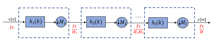
If M ≫ 1, the multistage approach reduces computational and storage requirements significantly.
Multistage Interpolator
Consider a J-stage interpolator. The overall interpolation factor L is split into smaller factors with each factor being the interpolation factor of the corresponding individual stage. The filter in each interpolator eliminates the images introduced by the upsampling process in the corresponding interpolator. The combined interpolation of all the individual stages must equal the overall interpolation. The combined response must meet or exceed the given design specifications.
The overall interpolation factor L is expressed as the product of smaller factors:
where Lj is the interpolation factor for stage j. Each stage is an independent interpolator. The sample rate at the output of each jth stage is:
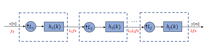
If L ≫ 1, the multistage approach reduces computational and storage requirements significantly.
Determine the number of stages and rate conversion factor for each stage
For a given rate conversion factor R, there is more than one possible configuration of filter stages. The number of stages and the rate conversion factor for each stage depends on the number of smaller factors R can be divided into. An optimal configuration is the sequence of filter stages leading to the least computational effort, with the computational effort measured by the number of multiplications per input sample, number of additions per input sample, and, in general, the total number of filter coefficients.
In the optimal configuration of multistage decimation filters, the shortest filter appears first and the longest filter (with the narrowest transition width) appears last. This sequence ensures that the filter with the longest length operates at the lowest sample rate, thereby reducing the cost of implementing the filter significantly.
Similarly, in the optimal configuration of multistage interpolation filters, the longest filter appears first and the shortest filter appears last. This sequence again ensures that the filter with the longest length operates at the lowest sample rate.
The designMultistageDecimator and designMultistageInterpolator functions in DSP System Toolbox™ automatically determine the optimal configuration, which includes
determining the number of stages and the rate conversion factor for each stage. An
optimal configuration leads to the least computational effort, and you can measure
the cost of such an implementation using the cost function. For an example, see
Multistage Rate Conversion.
See Also
Functions
Related Topics
You can also select a web site from the following list:
Americas
- América Latina (Español)
- Canada (English)
- United States (English)
Europe
- Belgium (English)
- Denmark (English)
- Deutschland (Deutsch)
- España (Español)
- Finland (English)
- France (Français)
- Ireland (English)
- Italia (Italiano)
- Luxembourg (English)
- Netherlands (English)
- Norway (English)
- Österreich (Deutsch)
- Portugal (English)
- Sweden (English)
- Switzerland
- United Kingdom (English)