Build a Map with Lidar Odometry and Mapping (LOAM) Using Unreal Engine Simulation

This example shows how to build a map with the lidar odometry and mapping (LOAM) [1] algorithm by using synthetic lidar data from the Unreal Engine® simulation environment. In this example, you learn how to:

• Record and visualize synthetic lidar sensor data from a 3D simulation environment using the Unreal Engine.

• Use the LOAM algorithm to register the recorded point clouds and build a map.

Set Up Scenario in Simulation Environment

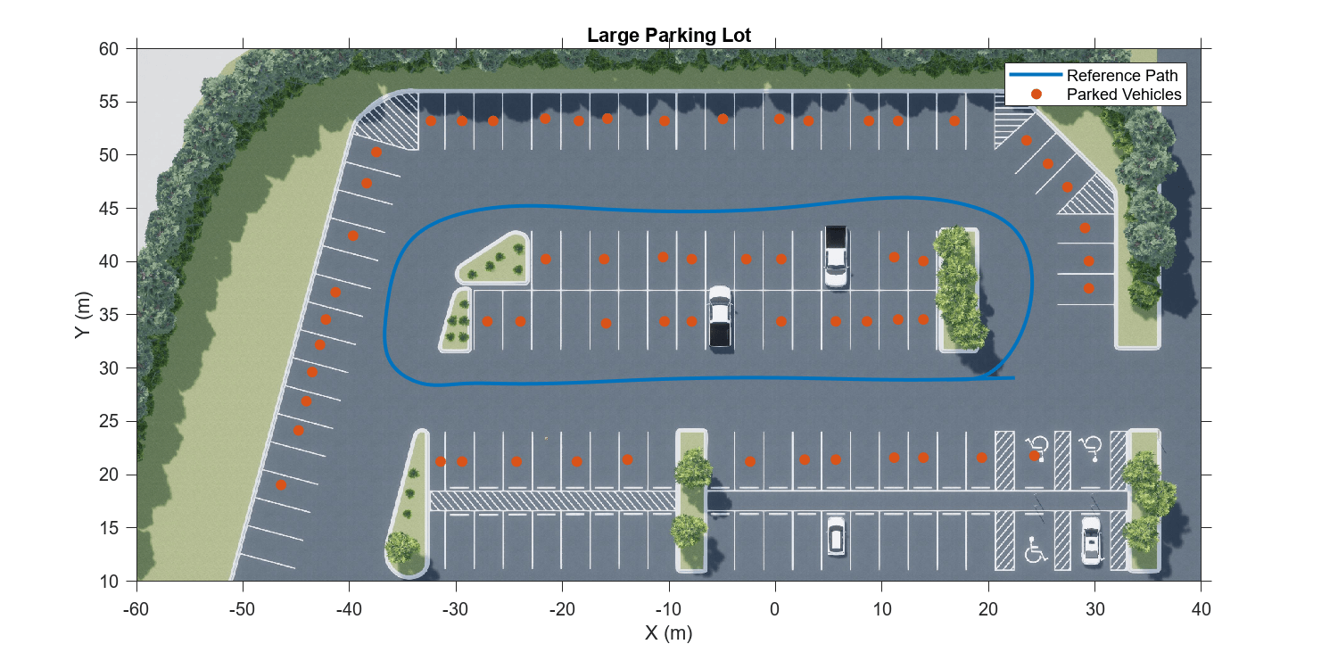
Load the prebuilt Large Parking Lot scene and a preselected reference trajectory. For information on how to generate a reference trajectory interactively by selecting a sequence of waypoints, see the Select Waypoints for Unreal Engine Simulation example.

% Load reference path
data = load("parkingLotReferenceData.mat");

% Set reference trajectory of the ego vehicle
refPosesX = data.refPosesX;
refPosesY = data.refPosesY;
refPosesT = data.refPosesT;

% Set poses of the parked vehicles
parkedPoses = data.parkedPoses;

% Display the reference trajectory and the parked vehicle locations
sceneName = "LargeParkingLot";
hScene = figure(Name="Large Parking Lot",NumberTitle="off");
helperShowSceneImage(sceneName);
hold on
plot(refPosesX(:,2),refPosesY(:,2),LineWidth=2,DisplayName="Reference Path");
scatter(parkedPoses(:,1),parkedPoses(:,2),[],"filled",DisplayName="Parked Vehicles");
xlim([-60 40])
ylim([10 60])
hScene.Position = [100 100 1000 500]; % Resize figure
title("Large Parking Lot")
legend

Open the Simulink® model, and add additional vehicles to the scene using the helperAddParkedVehicle function.

modelName = 'GenerateLidarDataOfParkingLot';
open_system(modelName)
snapnow
helperAddParkedVehicles(modelName,parkedPoses)

Record and Visualize Data

Use the Simulation 3D Vehicle with Ground Following block to simulate a vehicle moving along the specified reference trajectory. Use the Simulation 3D Lidar block to mount a lidar on the center of the roof of the vehicle, and record the sensor data.

close(hScene)

if ismac
    error(['3D Simulation is supported only on Microsoft' char(174) ' Windows' char(174) ' and Linux' char(174) '.']);
end

% Run simulation
simOut = sim(modelName);

close_system(modelName,0)

Use the helperGetPointClouds function and the helperGetLidarGroundTruth function to extract the lidar data and the ground truth poses.

ptCloudArr = helperGetPointClouds(simOut);
groundTruthPosesLidar = helperGetLidarGroundTruth(simOut);

Detect Edge Points and Surface Points

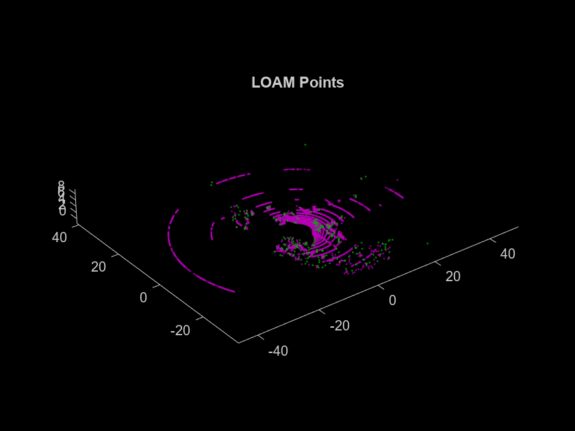
The LOAM algorithm uses edge points and surface points for registration and mapping. The detectLOAMFeatures (Lidar Toolbox) function outputs a LOAMPoints (Lidar Toolbox) object, which stores the selected edge points and surface points. It includes the label of each point, which can be sharp-edge, less-sharp-edge, planar-surface, or less-planar-surface. Use the pcregisterloam (Lidar Toolbox) function to register two organized point clouds.

ptCloud = ptCloudArr(1);
nextPtCloud = ptCloudArr(2);
gridStep = 0.5;
tform = pcregisterloam(ptCloud,nextPtCloud,gridStep);
disp(tform)

  rigidtform3d with properties:

    Dimensionality: 3
       Translation: [-1.9489 4.3717 -0.9680]
                 R: [3×3 single]

                 A: [0.9909   -0.1344   -0.0103   -1.9489
                     0.1340    0.9905   -0.0296    4.3717
                     0.0142    0.0280    0.9995   -0.9680
                          0         0         0    1.0000]

Alternatively, for more control over the trade-off between accuracy and speed, you can first detect the LOAM feature points, and then perform LOAM registration using pcregisterloam (Lidar Toolbox). These steps are recommended before LOAM registration:

1. Detect LOAM feature points using the detectLOAMFeatures (Lidar Toolbox) function.

2. Downsample the less planar surface points using the downsampleLessPlanar (Lidar Toolbox) object function. This step helps speed up registration using the pcregisterloam (Lidar Toolbox) function.

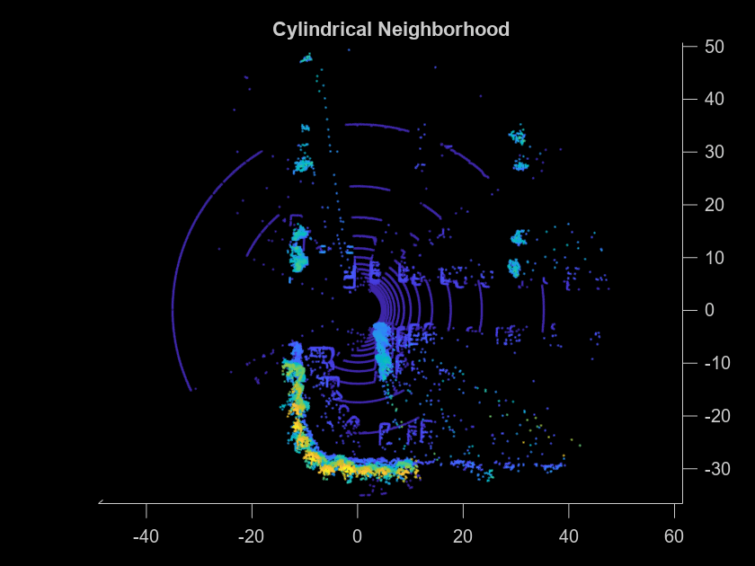
Because the detection algorithm relies on the neighbors of each point to classify edge points and surface points, as well as to identify unreliable points on the boundaries of occluded regions, preprocessing steps like downsampling, denoising and ground removal are not recommended before feature point detection. To remove noise from data farther from the sensor, and to speed up registration, filter the point cloud by range. The findPointsInCylinder object function selects a cylindrical neighborhood around the sensor, given a specified cylinder radius, and excludes data that is too close to the sensor and might include part of the vehicle.

egoRadius = 3.5;
cylinderRadius = 50;
selectedIdx = findPointsInCylinder(ptCloud,[egoRadius cylinderRadius]);
ptCloud = select(ptCloud,selectedIdx,OutputSize="full");
selectedIdx = findPointsInCylinder(nextPtCloud,[egoRadius cylinderRadius]);
nextPtCloud = select(nextPtCloud,selectedIdx,OutputSize="full");

figure
hold on
title("Cylindrical Neighborhood")
pcshow(ptCloud)
view(2)

Next, detect LOAM feature points using the detectLOAMFeatures (Lidar Toolbox) function. Tuning this function requires empirical analysis. The detectLOAMFeatures (Lidar Toolbox) name-value arguments provide a trade-off between registration accuracy and speed. To improve the accuracy of the registration, you must minimize the root mean squared error of the Euclidean distance between the aligned points. Track and minimize the root mean squared error output rmse of the pcregisterloam (Lidar Toolbox) function as you increase the value of the NumRegionsPerLaser, MaxSharpEdgePoints, MaxLessSharpEdgePoints, and MaxPlanarSurfacePoints arguments of detectLOAMFeatures (Lidar Toolbox).

maxPlanarSurfacePoints = 8;
points = detectLOAMFeatures(ptCloud,MaxPlanarSurfacePoints=maxPlanarSurfacePoints);
nextPoints = detectLOAMFeatures(nextPtCloud,MaxPlanarSurfacePoints=maxPlanarSurfacePoints);

figure
hold on
title("LOAM Points")
show(points,MarkerSize=12)

[~,rmseValue] = pcregisterloam(points,nextPoints);
disp(['RMSE: ' num2str(rmseValue)])

RMSE: 0.81254

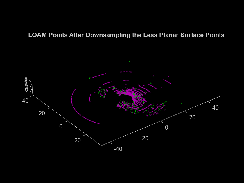
detectLOAMFeatures (Lidar Toolbox) first identifies sharp edge points, less sharp edge points, and planar surface points. All remaining points that are not considered unreliable points, and have a curvature value below the threshold are classified as less planar surface points. Downsampling the less planar surface points can speed up registration when using pcregisterloam (Lidar Toolbox).

points = downsampleLessPlanar(points,gridStep);

figure
hold on
title('LOAM Points After Downsampling the Less Planar Surface Points')
show(points,'MarkerSize',12)

Build Map Using Lidar Odometry

The LOAM algorithm consists of two main components that are integrated to compute an accurate transformation: Lidar Odometry and Lidar Mapping. Use the pcregisterloam (Lidar Toolbox) function with the one-to-one matching method to get the estimated transformation using the Lidar Odometry algorithm. The one-to-one matching method matches each point to its nearest neighbor, matching edge points to edge points and surface points to surface points. Use these matches to compute an estimate of the transformation. Use pcregisterloam (Lidar Toolbox) with the one-to-one matching method to incrementally build a map of the parking lot. Use a pcviewset object to manage the data.

Initialize the poses and the point cloud view set.

absPose = groundTruthPosesLidar(1);
relPose = rigidtform3d;
vSetOdometry = pcviewset;

Add the first view to the view set.

viewId = 1;
vSetOdometry = addView(vSetOdometry,viewId,absPose);

Register the point clouds incrementally and visualize the vehicle position in the parking lot scene.

% Display the parking lot scene with the reference trajectory
hScene = figure(Name="Large Parking Lot",NumberTitle="off");
helperShowSceneImage(sceneName);
hold on
plot(refPosesX(:,2),refPosesY(:,2),LineWidth=2)
xlim([-60 40])
ylim([10 60])
hScene.Position = [100 100 1000 500];

numSkip = 5;
for k = (numSkip+1):numSkip:numel(ptCloudArr)
    prevPoints = points;
    viewId = viewId + 1;
    ptCloud = ptCloudArr(k);

    % Select a cylindrical neighborhood of interest.
    selectedIdx = findPointsInCylinder(ptCloud,[egoRadius cylinderRadius]);
    ptCloud = select(ptCloud,selectedIdx,OutputSize="full");

    % Detect LOAM points and downsample the less planar surface points
    points = detectLOAMFeatures(ptCloud,MaxPlanarSurfacePoints=maxPlanarSurfacePoints);
    points = downsampleLessPlanar(points,gridStep);
    
    % Register the points using the previous relative pose as an initial
    % transformation
    relPose = pcregisterloam(points,prevPoints,InitialTransform=relPose);

    % Update the absolute pose and store it in the view set
    absPose = rigidtform3d(absPose.A * relPose.A);
    vSetOdometry = addView(vSetOdometry,viewId,absPose);

    % Visualize the absolute pose in the parking lot scene
    plot(absPose.Translation(1),absPose.Translation(2),Color="r",Marker=".",MarkerSize=8);
    xlim([-60 40])
    ylim([10 60])
    title("Build a Map Using Lidar Odometry")
    legend(["Ground Truth","Estimated Position"])
    pause(0.001)
    view(2)
end

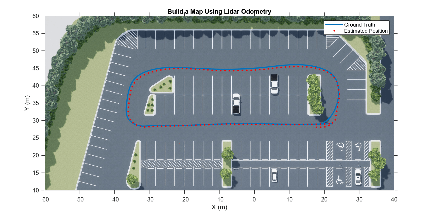
Improve the Accuracy of the Map with Lidar Mapping

Lidar Mapping refines the pose estimate from Lidar odometry by doing registration between points in a laser scan and points in a local map that includes multiple laser scans. It matches each point to multiple nearest neighbors in the local map, and then it uses these matches to refine the transformation estimate from Lidar odometry. Use the pcmaploam (Lidar Toolbox) object to manage the points in the map. Refine the pose estimates from Lidar odometry using findPose (Lidar Toolbox), and add points to the map using addPoints (Lidar Toolbox).

Initialize the poses.

absPose = groundTruthPosesLidar(1);
relPose = rigidtform3d;
vSetMapping = pcviewset;

Detect LOAM points in the first point cloud.

ptCloud = ptCloudArr(1);
selectedIdx = findPointsInCylinder(ptCloud,[egoRadius cylinderRadius]);
ptCloud = select(ptCloud,selectedIdx,OutputSize="full");
points = detectLOAMFeatures(ptCloud,'MaxPlanarSurfacePoints',maxPlanarSurfacePoints);
points = downsampleLessPlanar(points,gridStep);

Add the first view to the view set.

viewId = 1;
vSetMapping = addView(vSetMapping,viewId,absPose);

Create a map using the pcmaploam (Lidar Toolbox) class, and add points to the map using the addPoints (Lidar Toolbox) object function of pcmaploam (Lidar Toolbox).

voxelSize = 0.1;
loamMap = pcmaploam(voxelSize);
addPoints(loamMap,points,absPose);

Use pcregisterloam (Lidar Toolbox) with the one-to-one matching method to get an estimated pose using Lidar Odometry. Then, use the findPose (Lidar Toolbox) object function of pcmaploam (Lidar Toolbox) to find the absolute pose that aligns the points to the points in the map.

% Display the parking lot scene with the reference trajectory
hScene = figure(Name="Large Parking Lot",NumberTitle="off");
helperShowSceneImage(sceneName);
hold on
plot(refPosesX(:,2),refPosesY(:,2),LineWidth=2)
xlim([-60 40])
ylim([10 60])
hScene.Position = [100 100 1000 500];

for k = (numSkip+1):numSkip:numel(ptCloudArr)
    prevPtCloud = ptCloud;
    prevPoints = points;
    viewId = viewId + 1;
    ptCloud = ptCloudArr(k);

    % Select a cylindrical neighborhood of interest.
    selectedIdx = findPointsInCylinder(ptCloud,[egoRadius cylinderRadius]);
    ptCloud = select(ptCloud,selectedIdx,OutputSize="full");

    % Detect LOAM points and downsample the less planar surface points
    points = detectLOAMFeatures(ptCloud,MaxPlanarSurfacePoints=maxPlanarSurfacePoints);
    points = downsampleLessPlanar(points,gridStep);
    
    % Register the points using the previous relative pose as an initial
    % transformation
    relPose = pcregisterloam(points,prevPoints,MatchingMethod="one-to-one",InitialTransform=relPose);

    % Find the refined absolute pose that aligns the points to the map
    absPose = findPose(loamMap,points,relPose);

    % Store the refined absolute pose in the view set
    vSetMapping = addView(vSetMapping,viewId,absPose);

    % Add the new points to the map
    addPoints(loamMap,points,absPose);

    % Visualize the absolute pose in the parking lot scene
    plot(absPose.Translation(1),absPose.Translation(2),Color="r",Marker=".",MarkerSize=8)
    xlim([-60 40])
    ylim([10 60])
    title("Build a Map Using Lidar Mapping")
    legend(["Ground Truth","Estimated Position"])
    pause(0.001)
    view(2)
end

Compare Results

Visualize the estimated trajectories and compare them to the ground truth. Notice that combining Lidar Odometry and Lidar Mapping results in a more accurate map.

% Get the ground truth trajectory
groundTruthTrajectory = vertcat(groundTruthPosesLidar.Translation);

% Get the estimated trajectories
odometryPositions = vertcat(vSetOdometry.Views.AbsolutePose.Translation);
mappingPositions = vertcat(vSetMapping.Views.AbsolutePose.Translation);

% Plot the trajectories
figure
plot3(groundTruthTrajectory(:,1),groundTruthTrajectory(:,2),groundTruthTrajectory(:,3),LineWidth=2,DisplayName="Ground Truth")
hold on
plot3(odometryPositions(:,1),odometryPositions(:,2),odometryPositions(:,3),LineWidth=2,DisplayName="Odometry")
plot3(mappingPositions(:,1),mappingPositions(:,2),mappingPositions(:,3),LineWidth=2,DisplayName="Odometry and Mapping")
view(2)

legend
title("Compare Trajectories")

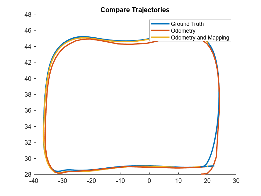
To numerically compare the estimated trajectories with the ground truth, compute the root-mean-square error (RMSE) between the ground truth trajectory and the estimated trajectory.

% Select the poses to compare
selectedGroundTruth = groundTruthTrajectory(1:numSkip:end,:);

% Compute the RMSE
rmseOdometry = rmse(selectedGroundTruth,odometryPositions,"all");
rmseWithMapping = rmse(selectedGroundTruth,mappingPositions,"all");
disp(['RMSE of the trajectory estimated with Odometry: ' num2str(rmseOdometry)])

RMSE of the trajectory estimated with Odometry: 1.0264

disp(['RMSE of the trajectory estimated with Odometry and Mapping: ' num2str(rmseWithMapping)])

RMSE of the trajectory estimated with Odometry and Mapping: 0.11836

References

[1] Zhang, Ji, and Sanjiv Singh. “LOAM: Lidar Odometry and Mapping in Real-Time.” In Robotics: Science and Systems X. Robotics: Science and Systems Foundation, 2014. https://doi.org/10.15607/RSS.2014.X.007.

Supporting Functions

helperGetPointClouds extracts an array of pointCloud objects that contain lidar sensor data.

function ptCloudArr = helperGetPointClouds(simOut)

% Extract signal
ptCloudData = simOut.ptCloudData.signals.values;

% Create a pointCloud array
ptCloudArr = pointCloud(ptCloudData(:,:,:,1));
for n = 2:size(ptCloudData,4)
    ptCloudArr(end+1) = pointCloud(ptCloudData(:,:,:,n));  %#ok<AGROW>
end

end

helperGetLidarGroundTruth extracts an array of rigidtform3d objects that contain the ground truth location and orientation.

function gTruth = helperGetLidarGroundTruth(simOut)

numFrames = size(simOut.lidarLocation.time,1);
gTruth = repmat(rigidtform3d,numFrames,1);

for i = 1:numFrames
    gTruth(i).Translation = squeeze(simOut.lidarLocation.signals.values(:,:,i));
    
    % Ignore the roll and the pitch rotations since the ground is flat
    yaw = double(simOut.lidarOrientation.signals.values(:,3,i));
    gTruth(i).R = [cos(yaw) -sin(yaw) 0;
                   sin(yaw)  cos(yaw) 0;
                      0         0     1];
end
end