Build a Map from Lidar Data

This example shows how to process 3-D lidar data from a sensor mounted on a vehicle to progressively build a map, with assistance from inertial measurement unit (IMU) readings. Such a map can facilitate path planning for vehicle navigation or can be used for localization. For evaluating the generated map, this example also shows how to compare the trajectory of the vehicle against global positioning system (GPS) recording.

Overview

High Definition (HD) maps are mapping services that provide precise geometry of roads up to a few centimeters in accuracy. This level of accuracy makes HD maps suitable for automated driving workflows such as localization and navigation. Such HD maps are generated by building a map from 3-D lidar scans, in conjunction with high-precision GPS and or IMU sensors and can be used to localize a vehicle within a few centimeters. This example implements a subset of features required to build such a system.

In this example, you learn how to:

• Load, explore and visualize recorded driving data

• Build a map using lidar scans

• Improve the map using IMU readings

Load and Explore Recorded Driving Data

The data used in this example is from this GitHub® repository, and represents approximately 100 seconds of lidar, GPS and IMU data. The data is saved in the form of MAT-files, each containing a timetable. Download the MAT-files from the repository and load them into the MATLAB® workspace.

Note: This download can take a few minutes.

baseDownloadURL = 'https://github.com/mathworks/udacity-self-driving-data-subset/raw/master/drive_segment_11_18_16/';
dataFolder      = fullfile(tempdir, 'drive_segment_11_18_16', filesep);
options         = weboptions('Timeout', Inf);

lidarFileName = dataFolder + "lidarPointClouds.mat";
imuFileName   = dataFolder + "imuOrientations.mat";
gpsFileName   = dataFolder + "gpsSequence.mat";

folderExists  = exist(dataFolder, 'dir');
matfilesExist = exist(lidarFileName, 'file') && exist(imuFileName, 'file') ...
    && exist(gpsFileName, 'file');

if ~folderExists
    mkdir(dataFolder);
end

if ~matfilesExist
    disp('Downloading lidarPointClouds.mat (613 MB)...')
    websave(lidarFileName, baseDownloadURL + "lidarPointClouds.mat", options);

    disp('Downloading imuOrientations.mat (1.2 MB)...')
    websave(imuFileName, baseDownloadURL + "imuOrientations.mat", options);

    disp('Downloading gpsSequence.mat (3 KB)...')
    websave(gpsFileName, baseDownloadURL + "gpsSequence.mat", options);
end

Downloading lidarPointClouds.mat (613 MB)...
Downloading imuOrientations.mat (1.2 MB)...
Downloading gpsSequence.mat (3 KB)...

First, load the point cloud data saved from a Velodyne® HDL32E lidar. Each scan of lidar data is stored as a 3-D point cloud using the pointCloud object. This object internally organizes the data using a K-d tree data structure for faster search. The timestamp associated with each lidar scan is recorded in the Time variable of the timetable.

% Load lidar data from MAT-file
data = load(lidarFileName);
lidarPointClouds = data.lidarPointClouds;

% Display first few rows of lidar data
head(lidarPointClouds)

        Time           PointCloud  
    _____________    ______________

    23:46:10.5115    1×1 pointCloud
    23:46:10.6115    1×1 pointCloud
    23:46:10.7116    1×1 pointCloud
    23:46:10.8117    1×1 pointCloud
    23:46:10.9118    1×1 pointCloud
    23:46:11.0119    1×1 pointCloud
    23:46:11.1120    1×1 pointCloud
    23:46:11.2120    1×1 pointCloud

Load the GPS data from the MAT-file. The Latitude, Longitude, and Altitude variables of the timetable are used to store the geographic coordinates recorded by the GPS device on the vehicle.

% Load GPS sequence from MAT-file
data = load(gpsFileName);
gpsSequence = data.gpsSequence;

% Display first few rows of GPS data
head(gpsSequence)

        Time         Latitude    Longitude    Altitude
    _____________    ________    _________    ________

    23:46:11.4563      37.4       -122.11      -42.5  
    23:46:12.4563      37.4       -122.11      -42.5  
    23:46:13.4565      37.4       -122.11      -42.5  
    23:46:14.4455      37.4       -122.11      -42.5  
    23:46:15.4455      37.4       -122.11      -42.5  
    23:46:16.4567      37.4       -122.11      -42.5  
    23:46:17.4573      37.4       -122.11      -42.5  
    23:46:18.4656      37.4       -122.11      -42.5  

Load the IMU data from the MAT-file. An IMU typically consists of individual sensors that report information about the motion of the vehicle. They combine multiple sensors, including accelerometers, gyroscopes and magnetometers. The Orientation variable stores the reported orientation of the IMU sensor. These readings are reported as quaternions. Each reading is specified as a 1-by-4 vector containing the four quaternion parts. Convert the 1-by-4 vector to a quaternion object.

% Load IMU recordings from MAT-file
data = load(imuFileName);
imuOrientations = data.imuOrientations;

% Convert IMU recordings to quaternion type
imuOrientations = convertvars(imuOrientations, 'Orientation', 'quaternion');

% Display first few rows of IMU data
head(imuOrientations)

        Time          Orientation  
    _____________    ______________

    23:46:11.4570    1×1 quaternion
    23:46:11.4605    1×1 quaternion
    23:46:11.4620    1×1 quaternion
    23:46:11.4655    1×1 quaternion
    23:46:11.4670    1×1 quaternion
    23:46:11.4705    1×1 quaternion
    23:46:11.4720    1×1 quaternion
    23:46:11.4755    1×1 quaternion

To understand how the sensor readings come in, for each sensor, compute the approximate frame duration.

lidarFrameDuration = median(diff(lidarPointClouds.Time));
gpsFrameDuration   = median(diff(gpsSequence.Time));
imuFrameDuration   = median(diff(imuOrientations.Time));

% Adjust display format to seconds
lidarFrameDuration.Format = 's';
gpsFrameDuration.Format   = 's';
imuFrameDuration.Format   = 's';

% Compute frame rates
lidarRate = 1/seconds(lidarFrameDuration);
gpsRate   = 1/seconds(gpsFrameDuration);
imuRate   = 1/seconds(imuFrameDuration);

% Display frame durations and rates
fprintf('Lidar: %s, %3.1f Hz\n', char(lidarFrameDuration), lidarRate);
fprintf('GPS  : %s, %3.1f Hz\n', char(gpsFrameDuration), gpsRate);
fprintf('IMU  : %s, %3.1f Hz\n', char(imuFrameDuration), imuRate);

Lidar: 0.10008 sec, 10.0 Hz
GPS  : 1.0001 sec, 1.0 Hz
IMU  : 0.002493 sec, 401.1 Hz

The GPS sensor is the slowest, running at a rate close to 1 Hz. The lidar is next slowest, running at a rate close to 10 Hz, followed by the IMU at a rate of almost 400 Hz.

Visualize Driving Data

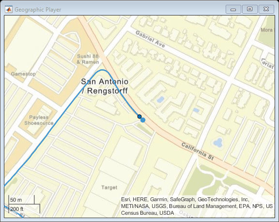
To understand what the scene contains, visualize the recorded data using streaming players. To visualize the GPS readings, use geoplayer. To visualize lidar readings using pcplayer.

% Create a geoplayer to visualize streaming geographic coordinates
latCenter = gpsSequence.Latitude(1);
lonCenter = gpsSequence.Longitude(1);
zoomLevel = 17;

gpsPlayer = geoplayer(latCenter, lonCenter, zoomLevel);

% Plot the full route
plotRoute(gpsPlayer, gpsSequence.Latitude, gpsSequence.Longitude);

% Determine limits for the player
xlimits = [-45 45]; % meters
ylimits = [-45 45];
zlimits = [-10 20];

% Create a pcplayer to visualize streaming point clouds from lidar sensor
lidarPlayer = pcplayer(xlimits, ylimits, zlimits);

% Customize player axes labels
xlabel(lidarPlayer.Axes, 'X (m)')
ylabel(lidarPlayer.Axes, 'Y (m)')
zlabel(lidarPlayer.Axes, 'Z (m)')

title(lidarPlayer.Axes, 'Lidar Sensor Data')

% Align players on screen
helperAlignPlayers({gpsPlayer, lidarPlayer});

% Outer loop over GPS readings (slower signal)
for g = 1 : height(gpsSequence)-1

    % Extract geographic coordinates from timetable
    latitude  = gpsSequence.Latitude(g);
    longitude = gpsSequence.Longitude(g);

    % Update current position in GPS display
    plotPosition(gpsPlayer, latitude, longitude);

    % Compute the time span between the current and next GPS reading
    timeSpan = timerange(gpsSequence.Time(g), gpsSequence.Time(g+1));

    % Extract the lidar frames recorded during this time span
    lidarFrames = lidarPointClouds(timeSpan, :);

    % Inner loop over lidar readings (faster signal)
    for l = 1 : height(lidarFrames)

        % Extract point cloud
        ptCloud = lidarFrames.PointCloud(l);

        % Update lidar display
        view(lidarPlayer, ptCloud);

        % Pause to slow down the display
        pause(0.01)
    end
end

Use Recorded Lidar Data to Build a Map

Lidars are powerful sensors that can be used for perception in challenging environments where other sensors are not useful. They provide a detailed, full 360 degree view of the environment of the vehicle.

% Hide players
hide(gpsPlayer)
hide(lidarPlayer)

% Select a frame of lidar data to demonstrate registration workflow
frameNum = 600;
ptCloud = lidarPointClouds.PointCloud(frameNum);

% Display and rotate ego view to show lidar data
helperVisualizeEgoView(ptCloud);

Lidars can be used to build centimeter-accurate HD maps, including HD maps of entire cities. These maps can later be used for in-vehicle localization. A typical approach to build such a map is to align successive lidar scans obtained from the moving vehicle and combine them into a single large point cloud. The rest of this example explores this approach to building a map.

1. Align lidar scans: Align successive lidar scans using a point cloud registration technique like the iterative closest point (ICP) algorithm or the normal-distributions transform (NDT) algorithm. See pcregistericp and pcregisterndt for more details about each algorithm. This example uses the Generalized-ICP (G-ICP) algorithm. The pcregistericp function returns the rigid transformation that aligns the moving point cloud with respect to the reference point cloud. By successively composing these transformations, each point cloud is transformed back to the reference frame of the first point cloud.

2. Combine aligned scans: Once a new point cloud scan is registered and transformed back to the reference frame of the first point cloud, the point cloud can be merged with the first point cloud using pcmerge.

Start by taking two point clouds corresponding to nearby lidar scans. To speed up processing, and accumulate enough motion between scans, use every tenth scan.

skipFrames = 10;
frameNum   = 100;

fixed  = lidarPointClouds.PointCloud(frameNum);
moving = lidarPointClouds.PointCloud(frameNum + skipFrames);

Downsample the point clouds prior to registration. Downsampling improves both registration accuracy and algorithm speed.

downsampleGridStep = 0.2;
fixedDownsampled  = pcdownsample(fixed, 'gridAverage', downsampleGridStep);
movingDownsampled = pcdownsample(moving, 'gridAverage', downsampleGridStep);

After preprocessing the point clouds, register them using the Generalized-ICP algorithm. This is available in pcregistericp by setting the Metric name-value argument to 'planeToPlane'. Visualize the alignment before and after registration.

regInlierRatio = 0.35;
tform = pcregistericp(movingDownsampled, fixedDownsampled, 'Metric', 'planeToPlane', ...
    'InlierRatio', regInlierRatio);

movingReg = pctransform(movingDownsampled, tform);

% Visualize alignment in top-view before and after registration
hFigAlign = figure;

subplot(121)
pcshowpair(movingDownsampled, fixedDownsampled)
title('Before Registration')
view(2)

subplot(122)
pcshowpair(movingReg, fixedDownsampled)
title('After Registration')
view(2)

helperMakeFigurePublishFriendly(hFigAlign);

Notice that the point clouds are well-aligned after registration. Even though the point clouds are closely aligned, the alignment is still not perfect.

Next, merge the point clouds using pcmerge.

mergeGridStep = 0.5;
ptCloudAccum = pcmerge(fixedDownsampled, movingReg, mergeGridStep);

hFigAccum = figure;
pcshow(ptCloudAccum)
title('Accumulated Point Cloud')
view(2)

helperMakeFigurePublishFriendly(hFigAccum);

Now that the processing pipeline for a single pair of point clouds is well-understood, put this together in a loop over the entire sequence of recorded data. The helperLidarMapBuilder class puts all this together. The updateMap method of the class takes in a new point cloud and goes through the steps detailed previously:

• Downsampling the point cloud.

• Estimating the rigid transformation required to merge the previous point cloud with the current point cloud.

• Transforming the point cloud back to the first frame.

• Merging the point cloud with the accumulated point cloud map.

Additionally, the updateMap method also accepts an initial transformation estimate, which is used to initialize the registration. A good initialization can significantly improve results of registration. Conversely, a poor initialization can adversely affect registration. Providing a good initialization can also improve the execution time of the algorithm.

A common approach to providing an initial estimate for registration is to use a constant velocity assumption. Use the transformation from the previous iteration as the initial estimate.

The updateDisplay method additionally creates and updates a 2-D top-view streaming point cloud display.

% Create a map builder object
mapBuilder = helperLidarMapBuilder('DownsampleGridStep', downsampleGridStep);

% Set random number seed
rng(0);

closeDisplay = false;
numFrames    = height(lidarPointClouds);

tform = rigidtform3d;
for n = 1 : skipFrames : numFrames - skipFrames + 1

    % Get the nth point cloud
    ptCloud = lidarPointClouds.PointCloud(n);

    % Use transformation from previous iteration as initial estimate for
    % current iteration of point cloud registration. (constant velocity)
    initTform = tform;

    % Update map using the point cloud
    tform = updateMap(mapBuilder, ptCloud, initTform);

    % Update map display
    updateDisplay(mapBuilder, closeDisplay);
end

Point cloud registration alone builds a map of the environment traversed by the vehicle. While the map may appear locally consistent, it might have developed significant drift over the entire sequence.

Use the recorded GPS readings as a ground truth trajectory, to visually evaluate the quality of the built map. First convert the GPS readings (latitude, longitude, altitude) to a local coordinate system. Select a local coordinate system that coincides with the origin of the first point cloud in the sequence. This conversion is computed using two transformations:

1. Convert the GPS coordinates to local Cartesian East-North-Up coordinates using the latlon2local function. The GPS location from the start of the trajectory is used as the reference point and defines the origin of the local x,y,z coordinate system.

2. Rotate the Cartesian coordinates so that the local coordinate system is aligned with the first lidar sensor coordinates. Since the exact mounting configuration of the lidar and GPS on the vehicle are not known, they are estimated.

% Select reference point as first GPS reading
origin = [gpsSequence.Latitude(1), gpsSequence.Longitude(1), gpsSequence.Altitude(1)];

% Convert GPS readings to a local East-North-Up coordinate system
[xEast, yNorth, zUp] = latlon2local(gpsSequence.Latitude, gpsSequence.Longitude, ...
    gpsSequence.Altitude, origin);

% Estimate rough orientation at start of trajectory to align local ENU
% system with lidar coordinate system
theta = median(atan2d(yNorth(1:15), xEast(1:15)));

R = [ cosd(90-theta) sind(90-theta) 0;
     -sind(90-theta) cosd(90-theta) 0;
     0               0              1];

% Rotate ENU coordinates to align with lidar coordinate system
groundTruthTrajectory = [xEast, yNorth, zUp] * R;

Superimpose the ground truth trajectory on the built map.

hold(mapBuilder.Axes, 'on')
scatter(mapBuilder.Axes, groundTruthTrajectory(:,1), groundTruthTrajectory(:,2), ...
    'green', 'filled');

helperAddLegend(mapBuilder.Axes, ...
    {'Map Points', 'Estimated Trajectory', 'Ground Truth Trajectory'});

Compare the estimated trajectory with the ground truth trajectory by computing the root-mean-square error (rmse) between the trajectories.

estimatedTrajectory = vertcat(mapBuilder.ViewSet.Views.AbsolutePose.Translation);
accuracyMetric = rmse(groundTruthTrajectory, estimatedTrajectory, 'all');

disp(['rmse between ground truth and estimated trajectory: ' num2str(accuracyMetric)])

rmse between ground truth and estimated trajectory: 9.773

After the initial turn, the estimated trajectory veers off the ground truth trajectory significantly. The trajectory estimated using point cloud registration alone can drift for a number of reasons:

• Noisy scans from the sensor without sufficient overlap

• Absence of strong enough features, for example, near long roads

• Inaccurate initial transformation, especially when rotation is significant

% Close map display
updateDisplay(mapBuilder, true);

Use IMU Orientation to Improve Built Map

An IMU is an electronic device mounted on a platform. IMUs contain multiple sensors that report various information about the motion of the vehicle. Typical IMUs incorporate accelerometers, gyroscopes, and magnetometers. An IMU can provide a reliable measure of orientation.

Use the IMU readings to provide a better initial estimate for registration. The IMU-reported sensor readings used in this example have already been filtered on the device.

% Reset the map builder to clear previously built map
reset(mapBuilder);

% Set random number seed
rng(0);

initTform = rigidtform3d;
for n = 1 : skipFrames : numFrames - skipFrames + 1

    % Get the nth point cloud
    ptCloud = lidarPointClouds.PointCloud(n);

    if n > 1
        % Since IMU sensor reports readings at a much faster rate, gather
        % IMU readings reported since the last lidar scan.
        prevTime = lidarPointClouds.Time(n - skipFrames);
        currTime = lidarPointClouds.Time(n);
        timeSinceScan = timerange(prevTime, currTime);

        imuReadings = imuOrientations(timeSinceScan, 'Orientation');

        % Form an initial estimate using IMU readings
        initTform = helperComputeInitialEstimateFromIMU(imuReadings, tform);
    end

    % Update map using the point cloud
    tform = updateMap(mapBuilder, ptCloud, initTform);

    % Update map display
    updateDisplay(mapBuilder, closeDisplay);
end

% Superimpose ground truth trajectory on new map
hold(mapBuilder.Axes, 'on')
scatter(mapBuilder.Axes, groundTruthTrajectory(:,1), groundTruthTrajectory(:,2), ...
    'green', 'filled');

helperAddLegend(mapBuilder.Axes, ...
    {'Map Points', 'Estimated Trajectory', 'Ground Truth Trajectory'});

% Capture snapshot for publishing
snapnow;

% Close open figures
close([hFigAlign, hFigAccum]);
updateDisplay(mapBuilder, true);

% Compare the trajectory estimated using the IMU orientation with the
% ground truth trajectory
estimatedTrajectory = vertcat(mapBuilder.ViewSet.Views.AbsolutePose.Translation);
accuracyMetricWithIMU = rmse(groundTruthTrajectory, estimatedTrajectory, 'all');

disp(['rmse between ground truth and trajectory estimated using IMU orientation: ' num2str(accuracyMetricWithIMU)])

rmse between ground truth and trajectory estimated using IMU orientation: 3.4613

Using the orientation estimate from IMU significantly improved registration, leading to a much closer trajectory with smaller drift.

Supporting Functions

helperAlignPlayers aligns a cell array of streaming players so they are arranged from left to right on the screen.

function helperAlignPlayers(players)

validateattributes(players, {'cell'}, {'vector'});

hasAxes = cellfun(@(p)isprop(p,'Axes'),players,'UniformOutput', true);
if ~all(hasAxes)
    error('Expected all viewers to have an Axes property');
end

screenSize   = get(groot, 'ScreenSize');
screenMargin = [50, 100];

playerSizes = cellfun(@getPlayerSize, players, 'UniformOutput', false);
playerSizes = cell2mat(playerSizes);

maxHeightInSet = max(playerSizes(1:3:end));

% Arrange players vertically so that the tallest player is 100 pixels from
% the top.
location = round([screenMargin(1), screenSize(4)-screenMargin(2)-maxHeightInSet]);
for n = 1 : numel(players)
    player = players{n};

    hFig = ancestor(player.Axes, 'figure');
    hFig.OuterPosition(1:2) = location;

    % Set up next location by going right
    location = location + [50+hFig.OuterPosition(3), 0];
end

    function sz = getPlayerSize(viewer)

        % Get the parent figure container
        h = ancestor(viewer.Axes, 'figure');

        sz = h.OuterPosition(3:4);
    end
end

helperVisualizeEgoView visualizes point cloud data in the ego perspective by rotating about the center.

function player = helperVisualizeEgoView(ptCloud)

% Create a pcplayer object
xlimits = ptCloud.XLimits;
ylimits = ptCloud.YLimits;
zlimits = ptCloud.ZLimits;

player = pcplayer(xlimits, ylimits, zlimits);

% Turn off axes lines
axis(player.Axes, 'off');

% Set up camera to show ego view
camproj(player.Axes, 'perspective');
camva(player.Axes, 90);
campos(player.Axes, [0 0 0]);
camtarget(player.Axes, [-1 0 0]);

% Set up a transformation to rotate by 5 degrees
theta = 5;

eulerAngles = [0 0 theta];
translation = [0 0 0];
rotateByTheta = rigidtform3d(eulerAngles, translation);

for n = 0 : theta : 359
    % Rotate point cloud by theta
    ptCloud = pctransform(ptCloud, rotateByTheta);

    % Display point cloud
    view(player, ptCloud);

    pause(0.05)
end
end

helperComputeInitialEstimateFromIMU estimates an initial transformation for registration using IMU orientation readings and previously estimated transformation.

function tform = helperComputeInitialEstimateFromIMU(imuReadings, prevTform)

% Initialize transformation using previously estimated transform
tform = prevTform;

% If no IMU readings are available, return
if height(imuReadings) <= 1
    return;
end

% IMU orientation readings are reported as quaternions representing the
% rotational offset to the body frame. Compute the orientation change
% between the first and last reported IMU orientations during the interval
% of the lidar scan.
q1 = imuReadings.Orientation(1);
q2 = imuReadings.Orientation(end);

% Compute rotational offset between first and last IMU reading by
%   - Rotating from q2 frame to body frame
%   - Rotating from body frame to q1 frame
q = q1 * conj(q2);

% Convert to Euler angles
yawPitchRoll = euler(q, 'ZYX', 'point');

% Discard pitch and roll angle estimates. Use only heading angle estimate
% from IMU orientation.
yawPitchRoll(2:3) = 0;

% Convert back to rotation matrix
q = quaternion(yawPitchRoll, 'euler', 'ZYX', 'point');
tform.R = rotmat(q, 'point');
end

helperAddLegend adds a legend to the axes.

function helperAddLegend(hAx, labels)

% Add a legend to the axes
hLegend = legend(hAx, labels{:});

% Set text color and font weight
hLegend.TextColor  = [1 1 1];
hLegend.FontWeight = 'bold';
end

helperMakeFigurePublishFriendly adjusts figures so that screenshot captured by publish is correct.

function helperMakeFigurePublishFriendly(hFig)

if ~isempty(hFig) && isvalid(hFig)
    hFig.HandleVisibility = 'callback';
end

end