Train Network Using Model Function
This example shows how to create and train a deep learning network by using functions rather than a layer graph or a dlnetwork. The advantage of using functions is the flexibility to describe a wide variety of networks. The disadvantage is that you must complete more steps and prepare your data carefully. This example uses images of handwritten digits, with the dual objectives of classifying the digits and determining the angle of each digit from the vertical.
Load Training Data
The digitTrain4DArrayData function loads the images, their digit labels, and their angles of rotation from the vertical. Create arrayDatastore objects for the images, labels, and angles, and then use the combine function to make a single datastore that contains all of the training data. Extract the class names and number of nondiscrete responses.
[XTrain,T1Train,T2Train] = digitTrain4DArrayData;

dsXTrain = arrayDatastore(XTrain,IterationDimension=4);
dsT1Train = arrayDatastore(T1Train);
dsT2Train = arrayDatastore(T2Train);

dsTrain = combine(dsXTrain,dsT1Train,dsT2Train);

classNames = categories(T1Train);
numClasses = numel(classNames);
numResponses = size(T2Train,2);
numObservations = numel(T1Train);
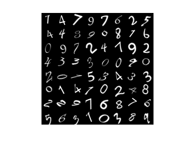
View some images from the training data.
idx = randperm(numObservations,64);
I = imtile(XTrain(:,:,:,idx));
figure
imshow(I)
Define Deep Learning Model
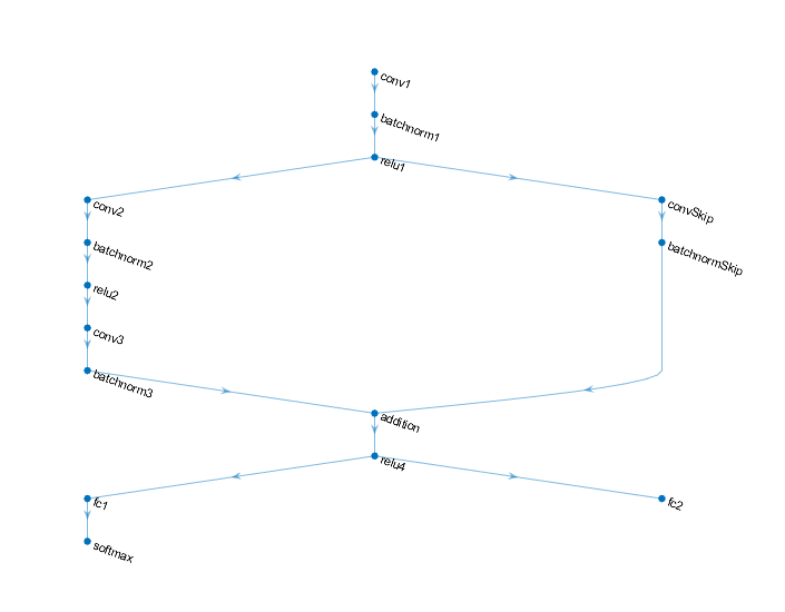
Define the following network that predicts both labels and angles of rotation.
A convolution-batchnorm-ReLU block with 16 5-by-5 filters.
A branch of two convolution-batchnorm blocks each with 32 3-by-3 filters with a ReLU operation between
A skip connection with a convolution-batchnorm block with 32 1-by-1 convolutions.
Combine both branches using addition followed by a ReLU operation
For the regression output, a branch with a fully connected operation of size 1 (the number of responses).
For classification output, a branch with a fully connected operation of size 10 (the number of classes) and a softmax operation.
Define and Initialize Model Parameters and State
Define the parameters for each of the operations and include them in a struct. Use the format parameters.OperationName.ParameterName where parameters is the struct, OperationName is the name of the operation (for example "conv1") and ParameterName is the name of the parameter (for example, "Weights").
Create a structure parameters containing the model parameters. Initialize the learnable weights and biases using the initializeGlorot and initializeZeros example functions, respectively. Initialize the batch normalization offset and scale parameters with the initializeZeros and initializeOnes example functions, respectively.
To perform training and inference using batch normalization operations, you must also manage the network state. Before prediction, you must specify the dataset mean and variance derived from the training data. Create a structure state containing the state parameters. The batch normalization statistics must not be dlarray objects. Initialize the batch normalization trained mean and trained variance states using the zeros and ones functions, respectively.
The initialization example functions are attached to this example as supporting files.
Initialize the parameters for the first convolution operation, "conv1".
filterSize = [5 5];
numChannels = 1;
numFilters = 16;

sz = [filterSize numChannels numFilters];
numOut = prod(filterSize) * numFilters;
numIn = prod(filterSize) * numFilters;

parameters.conv1.Weights = initializeGlorot(sz,numOut,numIn);
parameters.conv1.Bias = initializeZeros([numFilters 1]);
Initialize the parameters and state for the first batch normalization operation, "batchnorm1".
parameters.batchnorm1.Offset = initializeZeros([numFilters 1]);
parameters.batchnorm1.Scale = initializeOnes([numFilters 1]);
state.batchnorm1.TrainedMean = initializeZeros([numFilters 1]);
state.batchnorm1.TrainedVariance = initializeOnes([numFilters 1]);
Initialize the parameters for the second convolution operation, "conv2".
filterSize = [3 3];
numChannels = 16;
numFilters = 32;

sz = [filterSize numChannels numFilters];
numOut = prod(filterSize) * numFilters;
numIn = prod(filterSize) * numFilters;

parameters.conv2.Weights = initializeGlorot(sz,numOut,numIn);
parameters.conv2.Bias = initializeZeros([numFilters 1]);
Initialize the parameters and state for the second batch normalization operation, "batchnorm2".
parameters.batchnorm2.Offset = initializeZeros([numFilters 1]);
parameters.batchnorm2.Scale = initializeOnes([numFilters 1]);
state.batchnorm2.TrainedMean = initializeZeros([numFilters 1]);
state.batchnorm2.TrainedVariance = initializeOnes([numFilters 1]);
Initialize the parameters for the third convolution operation, "conv3".
filterSize = [3 3];
numChannels = 32;
numFilters = 32;

sz = [filterSize numChannels numFilters];
numOut = prod(filterSize) * numFilters;
numIn = prod(filterSize) * numFilters;

parameters.conv3.Weights = initializeGlorot(sz,numOut,numIn);
parameters.conv3.Bias = initializeZeros([numFilters 1]);
Initialize the parameters and state for the third batch normalization operation, "batchnorm3".
parameters.batchnorm3.Offset = initializeZeros([numFilters 1]);
parameters.batchnorm3.Scale = initializeOnes([numFilters 1]);
state.batchnorm3.TrainedMean = initializeZeros([numFilters 1]);
state.batchnorm3.TrainedVariance = initializeOnes([numFilters 1]);
Initialize the parameters for the convolution operation in the skip connection, "convSkip".
filterSize = [1 1];
numChannels = 16;
numFilters = 32;

sz = [filterSize numChannels numFilters];
numOut = prod(filterSize) * numFilters;
numIn = prod(filterSize) * numFilters;

parameters.convSkip.Weights = initializeGlorot(sz,numOut,numIn);
parameters.convSkip.Bias = initializeZeros([numFilters 1]);
Initialize the parameters and state for the batch normalization operation in the skip connection, "batchnormSkip".
parameters.batchnormSkip.Offset = initializeZeros([numFilters 1]);
parameters.batchnormSkip.Scale = initializeOnes([numFilters 1]);
state.batchnormSkip.TrainedMean = initializeZeros([numFilters 1]);
state.batchnormSkip.TrainedVariance = initializeOnes([numFilters 1]);
Initialize the parameters for the fully connected operation corresponding to the classification output, "fc1".
sz = [numClasses 6272];
numOut = numClasses;
numIn = 6272;
parameters.fc1.Weights = initializeGlorot(sz,numOut,numIn);
parameters.fc1.Bias = initializeZeros([numClasses 1]);
Initialize the parameters for the fully connected operation corresponding to the regression output, "fc2".
sz = [numResponses 6272];
numOut = numResponses;
numIn = 6272;
parameters.fc2.Weights = initializeGlorot(sz,numOut,numIn);
parameters.fc2.Bias = initializeZeros([numResponses 1]);
View the structure of the parameters.
parameters
parameters = struct with fields:
            conv1: [1×1 struct]
       batchnorm1: [1×1 struct]
            conv2: [1×1 struct]
       batchnorm2: [1×1 struct]
            conv3: [1×1 struct]
       batchnorm3: [1×1 struct]
         convSkip: [1×1 struct]
    batchnormSkip: [1×1 struct]
              fc1: [1×1 struct]
              fc2: [1×1 struct]
View the parameters for the "conv1" operation.
parameters.conv1
ans = struct with fields:
    Weights: [5×5×1×16 dlarray]
       Bias: [16×1 dlarray]
View the structure of the state parameters.
state
state = struct with fields:
       batchnorm1: [1×1 struct]
       batchnorm2: [1×1 struct]
       batchnorm3: [1×1 struct]
    batchnormSkip: [1×1 struct]
View the state parameters for the "batchnorm1" operation.
state.batchnorm1
ans = struct with fields:
        TrainedMean: [16×1 dlarray]
    TrainedVariance: [16×1 dlarray]
Define Model Function
Create the function model, listed at the end of the example, that computes the outputs of the deep learning model described earlier.
The function model takes the model parameters parameters, the input data, the flag doTraining which specifies whether to model should return outputs for training or prediction, and the network state. The network outputs the predictions for the labels, the predictions for the angles, and the updated network state.
Define Model Loss Function
Create the function modelLoss, listed at the end of the example, that takes the model parameters, a mini-batch of input data with corresponding targets containing the labels and angles, and returns the loss, the gradients of the loss with respect to the learnable parameters, and the updated network state.
Specify Training Options
Specify the training options. Train for 20 epochs with a mini-batch size of 128.
numEpochs = 20;
miniBatchSize = 128;
Train Model
Use minibatchqueue to process and manage the mini-batches of images. For each mini-batch:
Use the custom mini-batch preprocessing function
preprocessMiniBatch(defined at the end of this example) to one-hot encode the class labels.Format the image data with the dimension labels
"SSCB"(spatial, spatial, channel, batch). By default, theminibatchqueueobject converts the data todlarrayobjects with underlying typesingle. Do not add a format to the class labels or angles.Train on a GPU if one is available. By default, the
minibatchqueueobject converts each output to agpuArrayif a GPU is available. Using a GPU requires Parallel Computing Toolbox™ and a supported GPU device. For information on supported devices, see GPU Computing Requirements (Parallel Computing Toolbox).
mbq = minibatchqueue(dsTrain,...
    MiniBatchSize=miniBatchSize,...
    MiniBatchFcn=@preprocessMiniBatch,...
    MiniBatchFormat=["SSCB" "" ""]);
For each epoch, shuffle the data and loop over mini-batches of data. At the end of each iteration, display the training progress. For each mini-batch:
Evaluate the model loss and gradients using
dlfevaland themodelLossfunction.Update the network parameters using the
adamupdatefunction.
Initialize parameters for Adam.
trailingAvg = [];
trailingAvgSq = [];
To update the progress bar of the training progress monitor, calculate the total number of training iterations.
numIterationsPerEpoch = ceil(numObservations/miniBatchSize);
numIterations = numIterationsPerEpoch * numEpochs;
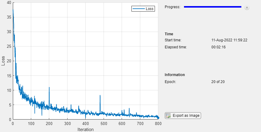
Initialize the TrainingProgressMonitor object. Because the timer starts when you create the monitor object, make sure that you create the object close to the training loop.
monitor = trainingProgressMonitor(Metrics="Loss",Info="Epoch",XLabel="Iteration");
Train the model.
epoch = 0;
iteration = 0;

% Loop over epochs.
while epoch < numEpochs && ~monitor.Stop
    epoch = epoch + 1;

    % Shuffle data.
    shuffle(mbq)

    % Loop over mini-batches
    while hasdata(mbq) && ~monitor.Stop

        iteration = iteration + 1;

        [X,T1,T2] = next(mbq);

        % Evaluate the model loss, gradients, and state, using dlfeval and the
        % modelLoss function.
        [loss,gradients,state] = dlfeval(@modelLoss,parameters,X,T1,T2,state);

        % Update the network parameters using the Adam optimizer.
        [parameters,trailingAvg,trailingAvgSq] = adamupdate(parameters,gradients, ...
            trailingAvg,trailingAvgSq,iteration);

        % Update the training progress monitor.
        recordMetrics(monitor,iteration,Loss=loss);
        updateInfo(monitor,Epoch=(epoch+" of "+numEpochs));
        monitor.Progress = 100 * iteration/numIterations;
    end
end
Test Model
Test the classification accuracy of the model by comparing the predictions on a test set with the true labels and angles. Manage the test data set using a minibatchqueue object with the same setting as the training data.
[XTest,T1Test,T2Test] = digitTest4DArrayData;

dsXTest = arrayDatastore(XTest,IterationDimension=4);
dsT1Test = arrayDatastore(T1Test);
dsT2Test = arrayDatastore(T2Test);

dsTest = combine(dsXTest,dsT1Test,dsT2Test);

mbqTest = minibatchqueue(dsTest,...
    MiniBatchSize=miniBatchSize,...
    MiniBatchFcn=@preprocessMiniBatch,...
    MiniBatchFormat=["SSCB" "" ""]);
To predict the labels and angles of the validation data, loop over the mini-batches and use the model function with the doTraining option set to false. Store the predicted classes and angles. Compare the predicted and true classes and angles and store the results.
doTraining = false;

classesPredictions = [];
anglesPredictions = [];
classCorr = [];
angleDiff = [];

% Loop over mini-batches.
while hasdata(mbqTest)

    % Read mini-batch of data.
    [X,T1,T2] = next(mbqTest);

    % Make predictions using the predict function.
    [Y1,Y2] = model(parameters,X,doTraining,state);

    % Determine predicted classes.
    Y1 = onehotdecode(Y1,classNames,1);
    classesPredictions = [classesPredictions Y1];

    % Dermine predicted angles
    Y2 = extractdata(Y2);
    anglesPredictions = [anglesPredictions Y2];

    % Compare predicted and true classes
    Y1Test = onehotdecode(T1,classNames,1);
    classCorr = [classCorr Y1 == Y1Test];

    % Compare predicted and true angles
    angleDiffBatch = Y2 - T2;
    angleDiff = [angleDiff extractdata(gather(angleDiffBatch))];
end
Evaluate the classification accuracy.
accuracy = mean(classCorr)
accuracy = 0.9848
Evaluate the regression accuracy.
angleRMSE = sqrt(mean(angleDiff.^2))
angleRMSE = single
    6.5363
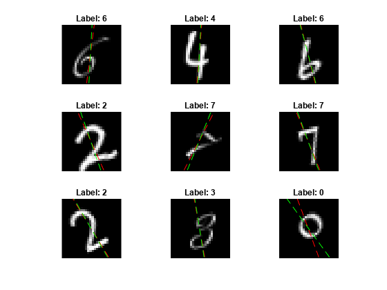
View some of the images with their predictions. Display the predicted angles in red and the correct labels in green.
idx = randperm(size(XTest,4),9);
figure
for i = 1:9
    subplot(3,3,i)
    I = XTest(:,:,:,idx(i));
    imshow(I)
    hold on

    sz = size(I,1);
    offset = sz/2;

    thetaPred = anglesPredictions(idx(i));
    plot(offset*[1-tand(thetaPred) 1+tand(thetaPred)],[sz 0],"r--")

    thetaValidation = T2Test(idx(i));
    plot(offset*[1-tand(thetaValidation) 1+tand(thetaValidation)],[sz 0],"g--")

    hold off
    label = string(classesPredictions(idx(i)));
    title("Label: " + label)
end
Model Function
The function model takes the model parameters parameters, the input data X, the flag doTraining which specifies whether to model should return outputs for training or prediction, and the network state state. The network outputs the predictions for the labels, the predictions for the angles, and the updated network state.

function [Y1,Y2,state] = model(parameters,X,doTraining,state)

% Initial operations
% Convolution - conv1
weights = parameters.conv1.Weights;
bias = parameters.conv1.Bias;
Y = dlconv(X,weights,bias,Padding="same");

% Batch normalization, ReLU - batchnorm1, relu1
offset = parameters.batchnorm1.Offset;
scale = parameters.batchnorm1.Scale;
trainedMean = state.batchnorm1.TrainedMean;
trainedVariance = state.batchnorm1.TrainedVariance;

if doTraining
    [Y,trainedMean,trainedVariance] = batchnorm(Y,offset,scale,trainedMean,trainedVariance);

    % Update state
    state.batchnorm1.TrainedMean = trainedMean;
    state.batchnorm1.TrainedVariance = trainedVariance;
else
    Y = batchnorm(Y,offset,scale,trainedMean,trainedVariance);
end

Y = relu(Y);


% Main branch operations
% Convolution - conv2
weights = parameters.conv2.Weights;
bias = parameters.conv2.Bias;
YnoSkip = dlconv(Y,weights,bias,Padding="same",Stride=2);

% Batch normalization, ReLU - batchnorm2, relu2
offset = parameters.batchnorm2.Offset;
scale = parameters.batchnorm2.Scale;
trainedMean = state.batchnorm2.TrainedMean;
trainedVariance = state.batchnorm2.TrainedVariance;

if doTraining
    [YnoSkip,trainedMean,trainedVariance] = batchnorm(YnoSkip,offset,scale,trainedMean,trainedVariance);

    % Update state
    state.batchnorm2.TrainedMean = trainedMean;
    state.batchnorm2.TrainedVariance = trainedVariance;
else
    YnoSkip = batchnorm(YnoSkip,offset,scale,trainedMean,trainedVariance);
end

YnoSkip = relu(YnoSkip);

% Convolution - conv3
weights = parameters.conv3.Weights;
bias = parameters.conv3.Bias;
YnoSkip = dlconv(YnoSkip,weights,bias,Padding="same");

% Batch normalization - batchnorm3
offset = parameters.batchnorm3.Offset;
scale = parameters.batchnorm3.Scale;
trainedMean = state.batchnorm3.TrainedMean;
trainedVariance = state.batchnorm3.TrainedVariance;

if doTraining
    [YnoSkip,trainedMean,trainedVariance] = batchnorm(YnoSkip,offset,scale,trainedMean,trainedVariance);

    % Update state
    state.batchnorm3.TrainedMean = trainedMean;
    state.batchnorm3.TrainedVariance = trainedVariance;
else
    YnoSkip = batchnorm(YnoSkip,offset,scale,trainedMean,trainedVariance);
end


% Skip connection operations
% Convolution, batch normalization (Skip connection) - convSkip, batchnormSkip
weights = parameters.convSkip.Weights;
bias = parameters.convSkip.Bias;
YSkip = dlconv(Y,weights,bias,Stride=2);

offset = parameters.batchnormSkip.Offset;
scale = parameters.batchnormSkip.Scale;
trainedMean = state.batchnormSkip.TrainedMean;
trainedVariance = state.batchnormSkip.TrainedVariance;

if doTraining
    [YSkip,trainedMean,trainedVariance] = batchnorm(YSkip,offset,scale,trainedMean,trainedVariance);

    % Update state
    state.batchnormSkip.TrainedMean = trainedMean;
    state.batchnormSkip.TrainedVariance = trainedVariance;
else
    YSkip = batchnorm(YSkip,offset,scale,trainedMean,trainedVariance);
end


% Final operations
% Addition, ReLU - addition, relu4
Y = YSkip + YnoSkip;
Y = relu(Y);

% Fully connect, softmax (labels) - fc1, softmax
weights = parameters.fc1.Weights;
bias = parameters.fc1.Bias;
Y1 = fullyconnect(Y,weights,bias);
Y1 = softmax(Y1);

% Fully connect (angles) - fc2
weights = parameters.fc2.Weights;
bias = parameters.fc2.Bias;
Y2 = fullyconnect(Y,weights,bias);

end
Model Loss Function
The modelLoss function, takes the model parameters, a mini-batch of input data X with corresponding targets T1 and T2 containing the labels and angles, respectively, and returns the loss, the gradients of the loss with respect to the learnable parameters, and the updated network state.
function [loss,gradients,state] = modelLoss(parameters,X,T1,T2,state)

doTraining = true;
[Y1,Y2,state] = model(parameters,X,doTraining,state);

lossLabels = crossentropy(Y1,T1);
lossAngles = mse(Y2,T2);

loss = lossLabels + 0.1*lossAngles;
gradients = dlgradient(loss,parameters);

end
Mini-Batch Preprocessing Function
The preprocessMiniBatch function preprocesses the data using the following steps:
Extract the image data from the incoming cell array and concatenate into a numeric array. Concatenating the image data over the fourth dimension adds a third dimension to each image, to be used as a singleton channel dimension.
Extract the label and angle data from the incoming cell arrays and concatenate along the second dimension into a categorical array and a numeric array, respectively.
One-hot encode the categorical labels into numeric arrays. Encoding into the first dimension produces an encoded array that matches the shape of the network output.
function [X,T1,T2] = preprocessMiniBatch(dataX,dataT1,dataT2)

    % Extract image data from cell and concatenate
    X = cat(4,dataX{:});
    % Extract label data from cell and concatenate
    T1 = cat(2,dataT1{:});
    % Extract angle data from cell and concatenate
    T2 = cat(2,dataT2{:});

    % One-hot encode labels
    T1 = onehotencode(T1,1);

end
See Also
dlarray | sgdmupdate | dlfeval | dlgradient | fullyconnect | dlconv | softmax | relu | batchnorm | crossentropy | minibatchqueue | onehotencode | onehotdecode
Topics
- Custom Loss Functions
- Custom Training Loops
- Custom Training Loop Model Loss Functions
- Train Generative Adversarial Network (GAN)
- Initialize Learnable Parameters for Model Function
- Update Batch Normalization Statistics Using Model Function
- Make Predictions Using Model Function
- Specify Training Options in Custom Training Loop
- List of Functions with dlarray Support