Train Complex-Valued Physics-Informed Neural Network

R2026b

Since R2026b

This example shows how to train a complex-valued, physics-informed neural network to simulate the behavior of electrons inside a simplified 2-D condensed matter physics system.

Physical quantities, such as temperature, angular momentum, or position, are real numbers. However, in quantum mechanics, the underlying quantity that describes the state of a physical system, known as the wave function, is complex valued. You can derive the real-valued physical quantities from the complex-valued wave function. To model the behavior of the wave function, and therefore the behavior of the observable physical quantities, in a quantum mechanical system, solve a complex-valued partial differential equation called the Schrödinger equation.

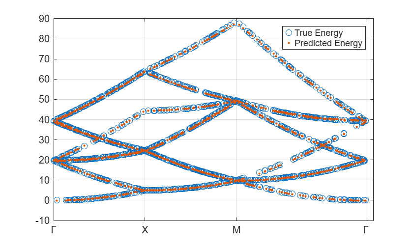
This example describes how to model a system of free electrons ($$V(r)=0$$) in a 2-D square crystal. For example, this plot shows the predicted energy of the free electrons compared with the true energy:

In a crystal, the Schrödinger equation simplifies to this complex partial differential equation:

$$\left[-\frac{1}{2}{\nabla }_r^2-ik\cdot {\nabla }_r+\frac{1}{2}{k}^2+V(r)\right]u_k(r)=E_k{u}_k(r).$$

Here, $$u_k(r)$$is the periodic part of the electron wave function, $$E_k$$ is the energy, $$r$$ is the real space coordinates, and $$k$$ is the reciprocal space coordinates, respectively. The reciprocal space coordinates are vectors that are input values to the wave function. For more information about the differential equation, see Bloch's theorem.

Following the work by Hsu et al. [1], model the system using two simple feedforward networks, one for the wave functions and one for energy. Connect the networks with a loss function that contains the Schrödinger equation and the periodic boundary conditions.

Create Training Data

In this network, the training data is composed of a single reciprocal space point $$k$$ for the energy network, and pairs of one real space point $$r$$ and one reciprocal space point $$k$$ for the wave function network.

To describe the energy, the energy network takes a single reciprocal space point $$k$$ as input and outputs the corresponding energy $$E_k$$. The training data for the energy network consists of a strategically chosen set of reciprocal space points.

To describe the wave function, the wave function network takes a real space point $$r$$ and a reciprocal space point $$k$$ as input and outputs the corresponding complex number $$u_k(r)$$. The training data for the wave function network consists of pairs of reciprocal and real space points.

First, define the crystal structure by defining the lattice constant, as well as the real space vectors, and the reciprocal lattice vectors. The real space lattice vectors define the periodicity of the crystal.

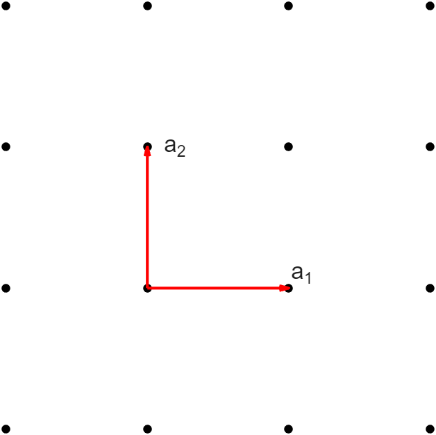
The lattice constant a is the length of the lattice vectors, and the reciprocal lattice vectors b1 and b2 are related to the real space lattice vectors a1 and a2 by the equation:

$$a_i\cdot b_j=2\pi {\delta }_{ij}.$$

Here, $${\delta }_{ij}$$ is the Kronecker delta, given by the equation:

$${\delta }_{ij}=\{\begin{array}{ll}1& \text{if}i=j,\\ 0& \text{if}i\ne j.\end{array}$$

Define the lattice constant and vectors.

crystalStructure.a = 1;
crystalStructure.a1 = crystalStructure.a * [1 0];
crystalStructure.a2 = crystalStructure.a * [0 1];
crystalStructure.b1 = 2*pi/crystalStructure.a * [1 0]; 
crystalStructure.b2 = 2*pi/crystalStructure.a * [0 1];

Create Reciprocal Space Points

Create nPoints reciprocal space points by using the reciprocalSpaceSampling function, which is attached to this example as a supporting file.

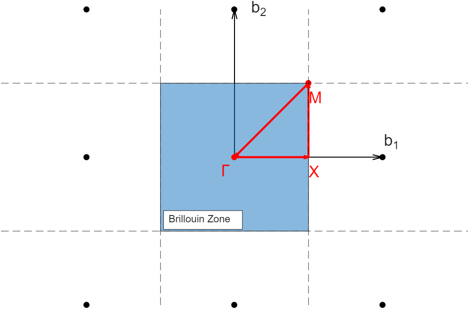
Take advantage of the crystal symmetry by sampling only from the irreducible Brillouin zone. The irreducible Brillouin zone is a subset of the Brillouin zone in reciprocal space that expresses the information contained in the entire Brillouin zone with fewer data points.

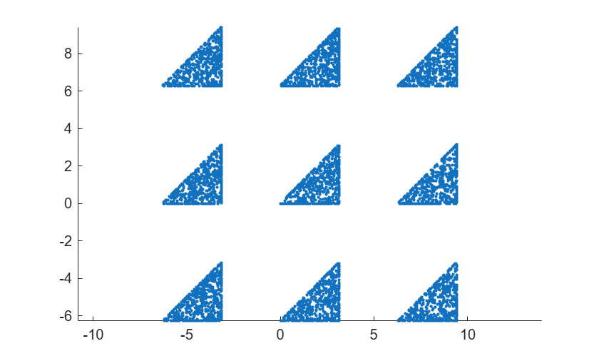
Sample from the irreducible Brillouin zone. Then, randomly shift some of the points by different reciprocal lattice vectors. This extended zone scheme increases the likelihood of the network generating higher-energy states.

Sample the first 30% of the reciprocal space points from the Brillouin zone path $$\Gamma \to X\to M\to \Gamma$$. For a square lattice, the Brillouin zone is also a square. $$\Gamma$$ is at the center of the square, $$X$$ is at the center of the right edge of the square, and $$M$$ is at the top right corner of the square. The path circumnavigates the irreducible Brillouin zone.

Create a vector that contains 5000 reciprocal space points.

crystalStructure.nPoints = 5000;

Create the reciprocal space points kPts and the relative position of the points bzBoundaryPosition along the Brillouin zone path by using the reciprocalSpaceSampling function, which is attached to this example as a supporting file.

[kPts,bzBoundaryPosition] = reciprocalSpaceSampling(crystalStructure);

Plot the reciprocal space points.

figure
scatter(kPts(:,1),kPts(:,2),'.')
axis equal

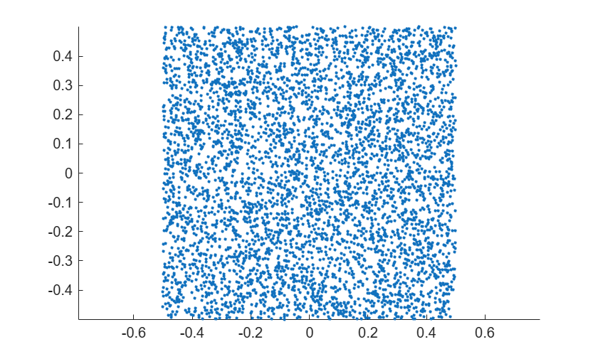
Create Real Space Points

Next, create nPoints real space points by randomly sampling them from the unit cell. To sample the real space points, use the realSpaceSampling function, which is attached to this example as a supporting file.

rPts = realSpaceSampling(crystalStructure);

Plot the real space points.

figure
scatter(rPts(:,1),rPts(:,2),'.')
axis equal

To create the training data set, concatenate the real and reciprocal space points into a single array.

XTrain = [rPts kPts];

Create Energy Network

This example uses two simple feedforward networks, one for the energy and one for the wave functions. Connect the networks with a loss function that contains the Schrödinger equation and the periodic boundary conditions, as illustrated in this diagram.

First, create the feedforward network for the energy. The network consists of four fullyConnectedLayer objects separated by swishLayer objects [1]. The fully connected layers in the energy network have output size 384.

The energy network takes two inputs $$k=(k_x,k_y)$$ and returns a single output $$E_k$$.

layersE = [
    featureInputLayer(2)        % Input: kx,ky
    fullyConnectedLayer(384)
    swishLayer
    fullyConnectedLayer(384)
    swishLayer
    fullyConnectedLayer(384)
    swishLayer
    fullyConnectedLayer(384)
    swishLayer
    fullyConnectedLayer(1)];    % Output: Ek 
netE = dlnetwork(layersE);

Create Custom Complex Activation Layer

The swishLayer object does not support complex-valued input data. Create a custom complex-valued swish layer to use in the wave function network.

Creating a custom layer that supports complex-valued input data follows the same process as creating a any other custom layer. Deep Learning Toolbox™ supports complex-valued automatic differentiation. To define a custom layer with complex-valued input, create the custom layer class and implement the forward function using complex-valued operations. If every operation in the forward function supports automatic differentiation, no further steps are required. Otherwise, implement the backward function manually by using the Wirtinger derivative.

To learn how to create custom layers, see Define Custom Deep Learning Layers.

The real-valued swish layer implements this activation function:

$$\text{swish}(x)=\frac{x}{1+\exp (-x)}.$$

To create a complex-valued swish layer that creates an equivalent network to the real-valued network in Hsu et al. [1], apply the swish activation separately to the real and imaginary parts of the input data:

$$\text{complexSwish}(z)=\text{swish}(\text{real}(z))+\text{i}\text{swish}(\text{imag}(z)).$$

The complex swish activation layer is attached to this example as a supporting file named complexSwishLayer.m.

classdef complexSwishLayer < nnet.layer.Layer & nnet.layer.Acceleratable
% complexSwishLayer   Complex-valued swish activation layer
%
%   A complex swish layer applies the swish activation function
%   separately to the real and imaginary parts of the input:
%
%       complexSwish(a + ib) = swish(a) + i*swish(b),
%
%   where swish(x) = x / (1 + exp(-x)).

    methods
        function layer = complexSwishLayer(args)
            arguments
                args.Name = "";
            end

            layer.Name = args.Name;
            layer.Description = "Complex Swish";
        end

        function Z = predict(~, X)
            Z = complex(swish(real(X)),swish(imag(X)));
        end
    end
end

function Y = swish(X)
    Y = X ./ (1 + exp(-X));
end

Create Complex-Valued Wave Function Network

The wave function network takes four inputs, $$k=(k_x,k_y)$$ and $$r=(x,y)$$ and returns a single complex output $$u_k(r)$$.

The multilayer perceptron part of the network consists of four complexFullyConnectedLayer objects separated by complexSwishLayer objects. The complex fully connected layers have output size 128.

To check that the wave functions satisfy the periodic boundary conditions in both real and reciprocal space, first map the input to a periodic coordinate representation by following the method from Shaviner et al.[3]. In a square lattice, the real space grid has a lattice constant of $$a$$, and the reciprocal lattice has a lattice constant of $$2\pi /a$$.

The equation for the periodic coordinate representation is:

$$\underset{}{\overset{\sim }{x}}=\left[\sin \left(\frac{2\pi }{a}x\right),\cos \left(\frac{2\pi }{a}x\right),\sin \left(\frac{2\pi }{a}y\right),\cos \left(\frac{2\pi }{a}y\right),\sin \left(a{k}_x\right),\cos \left(a{k}_x\right),\sin \left(a{k}_y\right),\cos \left(a{k}_y\right)\right].$$

Then, to remove spectral bias from the network, use a random Fourier feature to map the coordinates to a higher-dimensional space[3]:

$$\Phi (\underset{}{\overset{\sim }{x}})=\left[\sin (B\underset{}{\overset{\sim }{x}}),\cos (B\underset{}{\overset{\sim }{x}})\right],$$

where $$B$$ is a random 128-by-8 matrix. 128 is the output size of the subsequent fully connected layer, and 8 is the size of $$\underset{}{\overset{\sim }{x}}$$. Multiply the random variable by 2 to sample from a normal distribution with standard deviation 2.

B = 2*randn(128,8);

To perform these mappings, add two functionLayer objects to the beginning of the network. Specify the functions of the first functionLayer object as mapInputsToPeriodicCoordinates, and the function of the second object as randomFourierFeature. These functions are defined at the bottom of this example. Both functions support acceleration, so set the Acceleratable name-value argument to true.

layersU = [
    featureInputLayer(4)        % Input: x,y,kx,ky
    functionLayer(@(xTrain) mapInputsToPeriodicCoordinates(xTrain,crystalStructure.a),Acceleratable=true)
    functionLayer(@(xTilde) randomFourierFeature(xTilde,B),Acceleratable=true)
    complexFullyConnectedLayer(128)
    complexSwishLayer
    complexFullyConnectedLayer(128)
    complexSwishLayer
    complexFullyConnectedLayer(128)
    complexSwishLayer
    complexFullyConnectedLayer(128)
    complexSwishLayer
    complexFullyConnectedLayer(1)];    % Output: uk
netU = dlnetwork(layersU);

Create Loss Function

Many physics-informed neural networks incorporate the equations they are solving into their loss functions. For example, to solve a first-order differential equation of the form $$x^{\prime }=f(x,x^{\prime })$$, include the term $$|x^{\prime }-f(x,x^{\prime })|$$ in the loss function. The solutions to the differential equation minimize this loss term.

In this example, include two loss terms:

• Schrödinger function loss — The combined outputs of the two networks satisfies the Schrödinger equation, $$\left|\left[-\frac{1}{2}{\nabla }_r^2-ik\cdot {\nabla }_r+\frac{1}{2}{k}^2+V(r)\right]u_k(r)-E_k{u}_k(r)\right|.$$

• Normalization loss — The wave function network generates physically interesting non-zero wave functions when it satisfies the normalization condition: $${\int }_{\text{unit}\text{cell}}{u}_k^{*}(r)u_k(r){\text{d}}^{2}r=1.$$

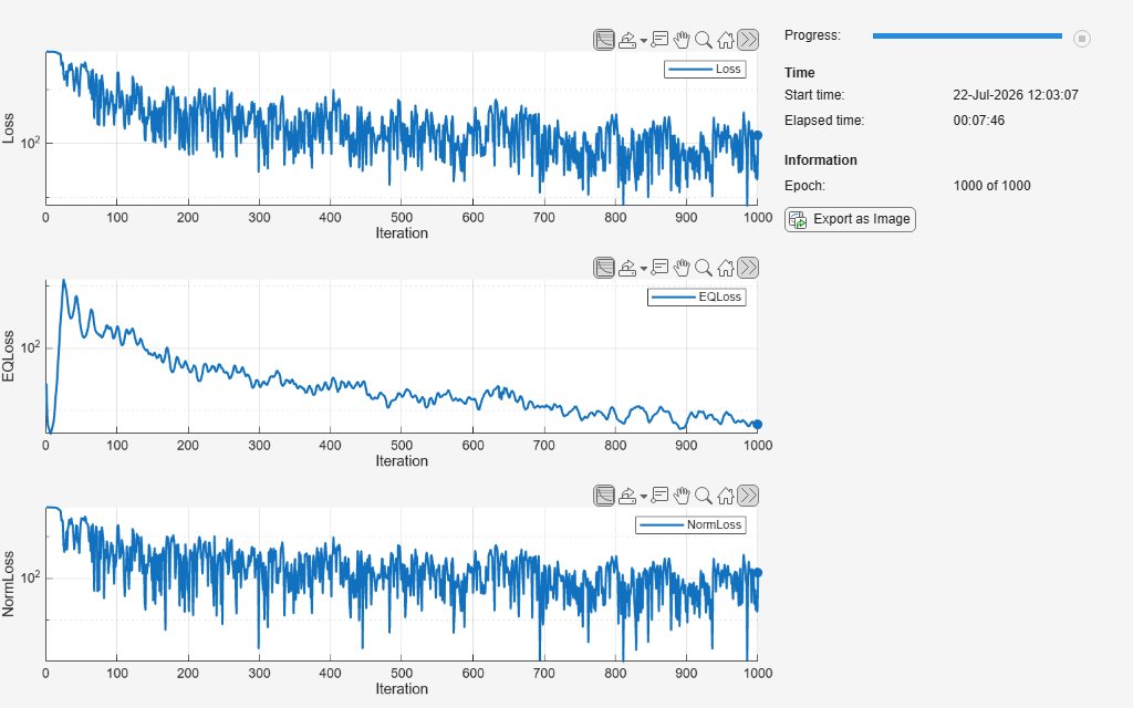
The two loss terms are weighted relative to each other. Choosing the weights requires empirical analysis. For this example, multiply the normalization loss term by a factor of 5000. To check if both loss terms contribute to the total loss, configure the training progress monitor to show the two loss terms separately in addition to the total loss term.

Specify the atomic pseudopotential, $$V(r)$$, using the atomicPseudoPotential function, which is attached to this example as a supporting file. This function takes the two real space coordinates x and y as inputs and returns the potential V(x,y). In this example, the potential is set to zero, $$V(r)=0$$.

To model a different atomic pseudo potential, you can adapt the atomicPseudoPotential function. Using a different potential can require different hyperparameters, such as different relative weights of the loss terms. Choosing hyperparameters requires empirical analysis. To explore different training option configurations by running experiments, you can use the Experiment Manager app.

To accelerate the loss function for the custom training loop by using the dlaccelerate function, include all loss terms in a single function.

function [loss,gradientsE,gradientsU,equationLoss,normalizationLoss] = lossTotal(netE,netU,X,crystalStructure)
x = X(1,:);
y = X(2,:);
kx = X(3,:);
ky = X(4,:);

To prevent complex numbers from leaking back into the real-valued energy network during backpropagation, convert the output of the energy network forward pass to real numbers.

E = real(forward(netE,[kx;ky]));
U = forward(netU,[x;y;kx;ky]);

a1 = crystalStructure.a1;
a2 = crystalStructure.a2;

%%% Schrödinger equation loss
V = atomicPseudoPotential(x,y);

U = stripdims(U);
x = stripdims(x);
y = stripdims(y);

Compute the derivative of the wave functions, U. The dlgradient function requires real-valued inputs, so differentiate the real and imaginary parts of U separately.

URealSumB = sum(real(U), 2);
UImagSumB = sum(imag(U), 2);
dUxReal = dlgradient(URealSumB,x,EnableHigherDerivatives=true);
dUxImag = dlgradient(UImagSumB,x,EnableHigherDerivatives=true);
dUyReal = dlgradient(URealSumB,y,EnableHigherDerivatives=true);
dUyImag = dlgradient(UImagSumB,y,EnableHigherDerivatives=true);

dUx = complex(dUxReal, dUxImag);
dUy = complex(dUyReal, dUyImag);

kineticEnergy = -0.5 * complex( ...
    dllaplacian(URealSumB,x,1) + dllaplacian(URealSumB,y,1), ...
    dllaplacian(UImagSumB,x,1) + dllaplacian(UImagSumB,y,1));
crystalMomentum = -1i*(kx.*dUx + ky.*dUy) + 0.5*(kx.^2 + ky.^2).*U;
atomicPotential = +V.*U;
eigenenergy = E.*U;

residual = kineticEnergy + crystalMomentum + atomicPotential - eigenenergy;

equationLoss = abs(residual).^2;
equationLoss = sum(equationLoss,2)/numel(x);

%%% Normalization loss
integrationResolution = 100;
integrationPoints = linspace(0,1,integrationResolution)' * a1 + linspace(0,1,integrationResolution)' * a2;
[XIntegration,YIntegration] = meshgrid(integrationPoints(:,1),integrationPoints(:,2));
XIntegration = reshape(XIntegration,1,[]);
YIntegration = reshape(YIntegration,1,[]);

kxForIntegral = kx(1) * ones(size(XIntegration));
kyForIntegral = ky(1) * ones(size(YIntegration));

UToIntegrate = forward(netU,[XIntegration; YIntegration; kxForIntegral; kyForIntegral]');
U2ToIntegrate = abs(UToIntegrate).^2;
U2ToIntegrate = reshape(U2ToIntegrate,integrationResolution,[]);

waveFunctionIntegral = trapezoidIntegral(integrationPoints(:,2),trapezoidIntegral(integrationPoints(:,1),U2ToIntegrate));   % custom integral function

normalizationLossWeight = 5e3;
normalizationLoss = normalizationLossWeight*abs(1 - waveFunctionIntegral);

loss = real(equationLoss + normalizationLoss);
[gradientsE,gradientsU] = dlgradient(loss,netE.Learnables,netU.Learnables);
end

Train Network

To train two networks connected by a single loss function, use a custom training loop. For another example of two networks connected by a shared loss, see Train Variational Autoencoder (VAE) to Generate Images.

Specify the training options. Train for 1000 epochs with a mini-batch size of 5000 and a learning rate of 0.001.

numEpochs = 1000;
miniBatchSize = 5000;
learnRate = 0.001;

Create a minibatchqueue object that processes and manages mini-batches of data during training. For each mini-batch:

• Convert the training data to an array data store

• Format the data with the dimension labels "BC" (batch, channel). By default, the minibatchqueue object converts the data to dlarray objects with the underlying type single.

• Train on a GPU if one is available. By default, the minibatchqueue object converts each output to a gpuArray if a GPU is available. Using a GPU requires Parallel Computing Toolbox™ and a supported GPU device. For information on supported devices, see GPU Computing Requirements (Parallel Computing Toolbox).

• To use only mini-batches that are all the same size, discard any partial mini-batches.

dsTrain = arrayDatastore(XTrain);
mbq = minibatchqueue(dsTrain, ...
    MiniBatchSize = miniBatchSize, ...
    MiniBatchFormat="BC", ...
    PartialMiniBatch="discard");

Initialize the parameters for the Adam solver.

trailingAvgE = [];
trailingAvgSqE = [];
trailingAvgU = [];
trailingAvgSqU = [];

Calculate the total number of iterations for the training progress monitor.

numObservationsTrain = size(XTrain,1);
numIterationsPerEpoch = ceil(numObservationsTrain / miniBatchSize);
numIterations = numEpochs * numIterationsPerEpoch;

Use the dlaccelerate function to speed up the evaluation of the model loss function lossTotal in the custom training loop.

crystalStructure = structfun(@dlarray,crystalStructure,UniformOutput=false);
lossFcn = dlaccelerate(@lossTotal);

Initialize the training progress monitor.

monitor = trainingProgressMonitor( ...
    Metrics=["Loss","EQLoss","NormLoss"], ...
    Info="Epoch", ...
    XLabel="Iteration");

Specify a logarithmic scale for the loss.

yscale(monitor,"Loss","log")
yscale(monitor,"EQLoss","log")
yscale(monitor,"NormLoss","log")

Train the network by using a custom training loop. For each epoch, shuffle the data and loop over mini-batches of data. For each mini-batch:

• Evaluate the model loss and gradients by using the dlfeval function.

• Update the wave function and energy network parameters by using the adamupdate function.

• Display the training progress.

epoch = 0;
iteration = 0;
% Loop over epochs.
while epoch < numEpochs && ~monitor.Stop
    epoch = epoch + 1;

    % Shuffle data.
    shuffle(mbq);

    % Loop over mini-batches.
    while hasdata(mbq) && ~monitor.Stop
        iteration = iteration + 1;

        % Read mini-batch of data.
        X = next(mbq);

        % Evaluate loss and gradients.
        [loss,gradientsE,gradientsU,eqLoss,normLoss] = dlfeval(lossFcn,netE,netU,X,crystalStructure);

        % Update learnable parameters.
        [netE,trailingAvgE,trailingAvgSqE] = adamupdate(netE, ...
            gradientsE,trailingAvgE,trailingAvgSqE,iteration,learnRate);

        [netU, trailingAvgU, trailingAvgSqU] = adamupdate(netU, ...
            gradientsU,trailingAvgU,trailingAvgSqU,iteration,learnRate);

        % Update the training progress monitor. 
        recordMetrics(monitor,iteration,Loss=loss,EQLoss=eqLoss,NormLoss=normLoss);
        updateInfo(monitor,Epoch=epoch + " of " + numEpochs);
        monitor.Progress = 100*iteration/numIterations;
    end
end

Test Network

Calculate the energies and plot the band structure along the reciprocal space path $$\Gamma \to X\to M\to \Gamma$$ by using the plotBandStructure function, which is attached to this example as a supporting file. The plotBandStructure function plots the energies computes by the trained neural network and compares it to the true, analytically known solution for free electrons.

E = forward(netE,kPts);
plotBandStructure(kPts,E,bzBoundaryPosition)

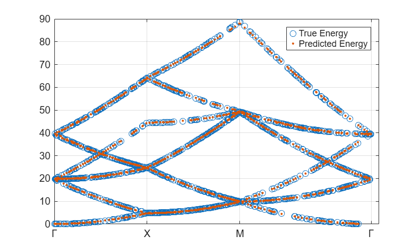
The predicted energies are very close to the true energy.

Next, plot the lowest-energy wave function at the center of the first Brillouin zone in a single unit cell by using the plotWaveFunction function, which is attached to this example as a supporting file. For free electrons, the periodic part of the electron wave function, $$u_k(r)$$, is constant.

k = [0 0];
plotWaveFunction(k,netU,crystalStructure)

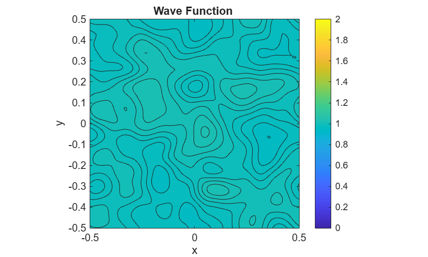
The periodic part of the wave function is close to being constant, as expected.

Supporting Functions

The mapInputsToPeriodicCoordinates function maps the real space and reciprocal space inputs to a periodic coordinate representation [3].

function xTilde = mapInputsToPeriodicCoordinates(xTrain,a)

x = xTrain(1,:);
y = xTrain(2,:);
kx = xTrain(3,:);
ky = xTrain(4,:);

Lk = 2*pi/a;
xTilde = dlarray(zeros(8,size(x,2)));
xTilde(1,:) = sin(2*pi/a*x);
xTilde(2,:) = cos(2*pi/a*x);
xTilde(3,:) = sin(2*pi/a*y);
xTilde(4,:) = cos(2*pi/a*y);
xTilde(5,:) = sin(2*pi/Lk*kx);
xTilde(6,:) = cos(2*pi/Lk*kx);
xTilde(7,:) = sin(2*pi/Lk*ky);
xTilde(8,:) = cos(2*pi/Lk*ky);
end

The randomFourierFeature function maps the periodic coordinates to a higher-dimensional complex space [3].

function phi = randomFourierFeature(xTilde,B)
phi = complex(cos(B*xTilde), sin(B*xTilde));
end

The trapezoidIntegral function computes the trapezoidal numerical integration of the dlarray object f with respect to variable x. To compute the trapezoidal numerical integration of a numerical array, use the trapz function instead. To calculate a two-dimensional integral, nest function calls to trapezoidIntegral, similar to trapz. For more information, see the Multiple Numerical Integrations example.

function Q = trapezoidIntegral(x,f)
if isvector(f) % assume dimensions: x n-by-1, f 1-by-n
    Q = (x(2:end) - x(1:end-1)).' * (f(1:end-1) + f(2:end)).'/2;
else % assume dimensions: x n-by-1, f n-by-n
    Q = (x(2:end) - x(1:end-1)).' * (f(1:end-1,:) + f(2:end,:))/2;
end
end

References

[1] Hsu, C., M. Mattheakis, G. R. Schleder, and D. T. Larson. "Equation-driven Neural Networks for Periodic Quantum Systems". Machine Learning and the Physical Sciences Workshop, NeurIPS 2024. https://ml4physicalsciences.github.io/2024/files/NeurIPS_ML4PS_2024_165.pdf

[2] https://github.com/circee/blochnet

[3] Shaviner, G. G., H. Chandravamsi, S. Pisnoy, Z. Chen, and S. H. Frankel. "PINNs for Solving Unsteady Maxwell's Equations: Convergence Issues and Comparative Assessment with Compact Schemes". ArXiv. https://arxiv.org/pdf/2504.12144