Get Started with Time Series Forecasting
This example shows how to create a simple long short-term memory (LSTM) network to model time series data using the Time Series Modeler app.
Time series forecasting involves predicting future values based on previously observed data points collected over time. You can train a deep learning model for time series forecasting using architectures such as recurrent neural networks (for example, LSTM or GRU networks) or feedforward networks (for example, multi-layer perceptron or convolutional neural networks).
Load Data
When you train a time series model, there are two types of input data you can use.
Responses: The time series you want to predict.
Predictors: These are external (exogenous) time series that influence the responses, but which you do not want to predict. Predictors are optional, and you can train autoregressive models using only responses.
Load example engine data. The model learns to predict values of a single response, engine torque, using four predictors: throttle position, wastegate valve area, engine speed, and spark timing.
load SIEngineDataOpen the Time Series Modeler app. In the Apps gallery, click Time Series Modeler.
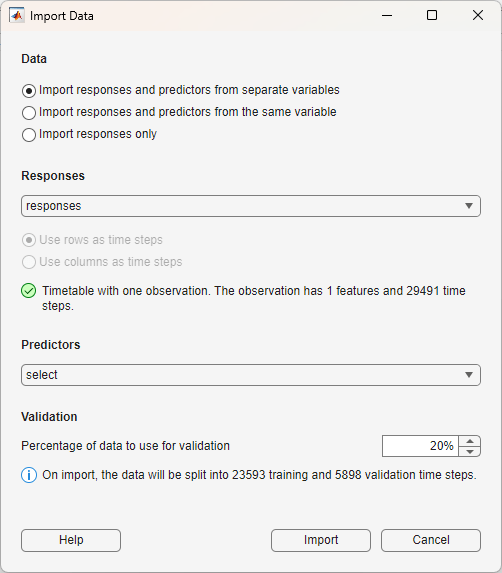
To import the data into the app, click New. The Import Data dialog box opens. In the dialog box, select Data to be Import responses and predictors from separate variables. Select the responses to be the responses variable. For the predictors, select the predictors variable. Use 20% of the data for validation and 80% for training.
Click Import.
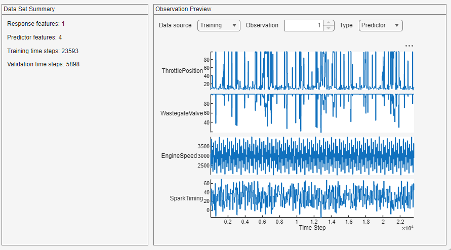
The app displays a summary of the data set and a preview of individual observations from the training and validation data, for both the responses and the predictors. You can select the data source to be the training or validation data, you can also select which observation to preview.
Select Model
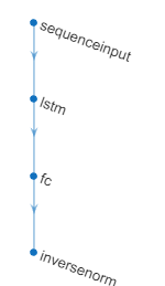
Select a deep learning model from the Model gallery. The model you should select depends on your task. For this example, select LSTM (Small). By default, this network has four layers. You can use the app to change the depth of the network and the number of learnable parameters (hidden units).
Train Model
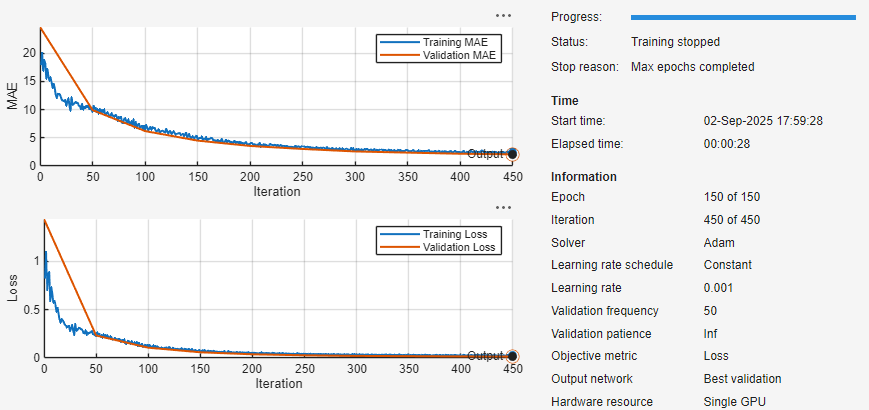
To train the model, click Train. During training, the app displays training information, plots of the mean absolute error (MAE) and loss (RMSE), and training diagnostics.
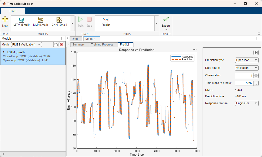
Test Model
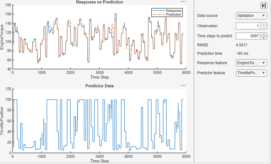
To use the model to forecast values, click Predict. For the selected observation, the app displays the true values and the predicted values. You can also see the RMSE value for the trained model. This value indicates how well the model performs on the validation data.
Export Model
When you are happy with the performance of your trained model, you can export it and use it on new test data. To export the model and generate code to forecast new values for test data, click Export.
See Also
dlnetwork | trainingOptions | trainnet | scores2label | Deep Network
Designer