Multivariate Time Series Anomaly Detection Using Graph Neural Network
This example shows how to detect anomalies in multivariate time series data using a graph neural network (GNN).
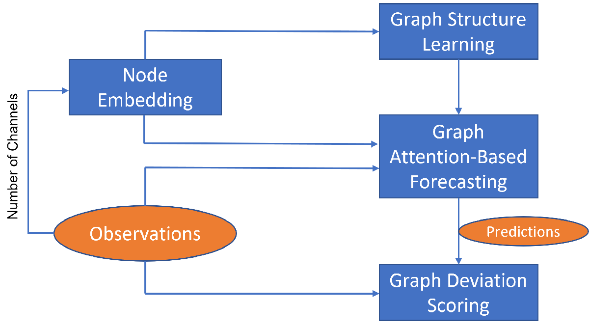
To detect anomalies or anomalous variables/channels in a multivariate time series data, you can use Graph Deviation Network (GDN) [1]. GDN is a type of GNN that learns a graph structure representing relationship between channels in a time series and detects anomalous channels and times by identifying deviations from the learned structure. GDN consists of four main components:
Node embedding: Generate learned embedding vectors to represent unique characteristics of each node/variable/channel.
Graph structure learning: Compute similarities between node embedding and use it to generate adjacency matrix representing learned graph structure.
Graph attention-based forecasting: Predict future values using graph attention.
Graph deviation scoring: Compute anomalous scores and identify anomalous nodes and time.
The components are illustrated in the figure below.
This example uses the human activity data, which consists of 24,075 time steps with 60 channels, for anomaly detection. The data set is not labeled with anomalies. Hence, the workflow described in this example is unsupervised anomaly detection.
Note: Training a GDN is a computationally intensive task. To make the example run quicker, this example skips the training step and loads a pretrained model. To instead train the model, set the doTraining variable to true.
doTraining = false;
Load Data
Load the human activity data. The data contains the variable feat, which is a numTimeSteps-by-numChannels array containing the time series data.
load humanactivityView the number of time steps and number of channels in feat.
[numTimeSteps,numChannels] = size(feat)
numTimeSteps = 24075
numChannels = 60
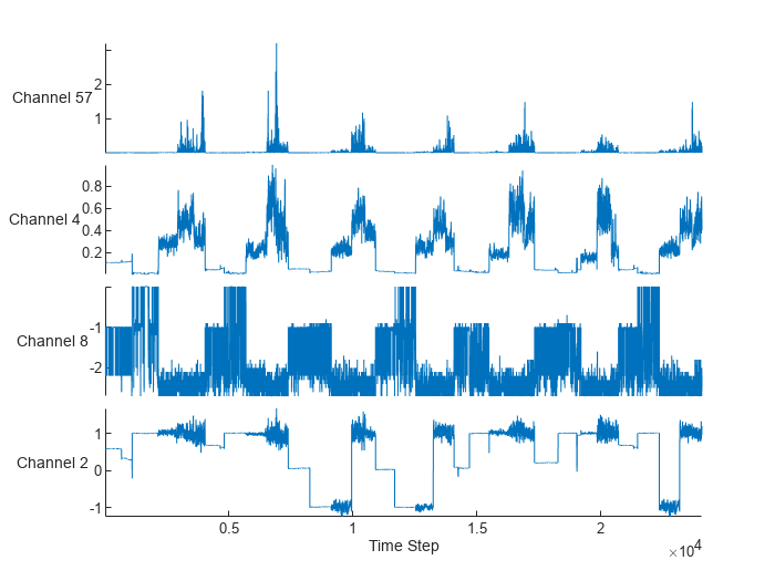
Randomly select and visualize four channels.
idx = randperm(numChannels,4);
figure
stackedplot(feat(:,idx),DisplayLabels="Channel " + idx);
xlabel("Time Step")
Prepare Data for Training
Partition the data using the first 40% time steps for training.
numTimeStepsTrain = floor(0.4*numTimeSteps);
numTimeStepsValidation = floor(0.2*numTimeSteps);

featuresTrain = feat(1:numTimeStepsTrain,:);
Normalize the training data.
[featuresTrain,muData,sigmaData] = normalize(featuresTrain);
To predict future values, input observations to the graph attention-based forecasting model are historical time series data based on a sliding window. Specify a sliding window size of 10.
windowSize = 10;
Obtain predictors and targets for the training data using the processData function defined in the Process Data section of the example. The function processes the data such that each time step is an observation and the predictors for each observation are the historical time series data of size windowSize-by-numChannels, and the targets are the numChannels-by-1 data of that time step.
[XTrain,TTrain] = processData(featuresTrain,windowSize);
View the size of the predictors.
size(XTrain)
ans = 1×3

          10          60        9620
View the size of the targets.
size(TTrain)
ans = 1×2

          60        9620
To train using minibatches of data, create an array datastore for the predictors and targets and combine them.
dsXTrain = arrayDatastore(XTrain,IterationDimension=3);
dsTTrain = arrayDatastore(TTrain,IterationDimension=2);
dsTrain = combine(dsXTrain,dsTTrain);
Define Model
Define the model. The model takes as input the predictor X and outputs predictions of the future values Y.
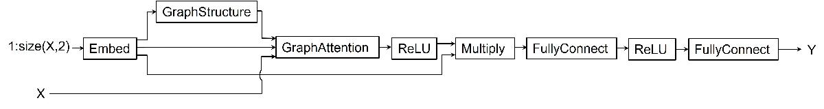
The model generates an embedding for each channel in the predictor
X.The model uses the embedding as input to a graph structure operation to generate adjacency matrix representing relations between channels.
Using the predictors, generated embedding, and adjacency matrix as input to a graph attention operation, the model computes graph embedding.
Finally, the model uses ReLU activation, multiply operation, and two fully connected operations with a ReLU activation in between to compute predictions for each channel in the predictors.
Initialize Model Parameters
Define the parameters for the each of the operations and include them in a structure. Use the format parameters.OperationName.ParameterName, where parameters is the struct, OperationName is the name of the operation (for example "fc"), and ParameterName is the name of the parameter (for example, "weights").
Create a structure to contain the learnable parameters for the model.
parameters = struct;
Set the hyperparameters. These include the top k number, which the graph structure operation uses to select the top k number of channels with highest similarity scores when computing channel relations. Set the top k number to 15.
topKNum = 15;
embeddingDimension = 96;
numHiddenUnits = 1024;
inputSize = numChannels+1;
Initialize the learnable parameters for the embed operation using the initializeGaussian function attached to the example as a supporting file. To access the function, open the example as a live script.
sz = [embeddingDimension inputSize];
mu = 0;
sigma = 0.01;
parameters.embed.weights = initializeGaussian(sz,mu,sigma);
Initialize the learnable parameters for the graph attention operation using the initializeGlorot and initializeZeros functions attached to the example as supporting files. To access these functions, open the example as a live script.
sz = [embeddingDimension windowSize];
numOut = embeddingDimension;
numIn = windowSize;

parameters.graphattn.weights.linear = initializeGlorot(sz,numOut,numIn);
attentionValueWeights = initializeGlorot([2 numOut],1,2*numOut);
attentionEmbedWeights = initializeZeros([2 numOut]);
parameters.graphattn.weights.attention = cat(2,attentionEmbedWeights,attentionValueWeights);
Initialize the weights for the fully connect operations using the initializeGlorot function, and the biases using the initializeZeros function.
sz = [numHiddenUnits embeddingDimension*numChannels];
numOut = numHiddenUnits;
numIn = embeddingDimension*numChannels;
parameters.fc1.weights = initializeGlorot(sz,numOut,numIn);
parameters.fc1.bias = initializeZeros([numOut,1]);

sz = [numChannels,numHiddenUnits];
numOut = numChannels;
numIn = numHiddenUnits;
parameters.fc2.weights = initializeGlorot(sz,numOut,numIn);
parameters.fc2.bias = initializeZeros([numOut,1]);
Define Model Function
Create the function model, defined in the Model Function section of the example, which takes as input the model parameters, the predictors for each time step, and the top k number, and returns predictions of future values.
Define Model Loss Function
Create the function modelLoss, defined in the Model Loss Function section of the example, which takes the model parameters, predictors, targets, and top k number, and returns the loss, the gradients of the loss with respect to the learnable parameters, and the model predictions.
Specify Training Options
Train for 80 epochs with a mini-batch size of 200 and set the learning rate for the Adam solver to 0.001.
numEpochs = 80;
miniBatchSize = 200;
learnRate = 0.001;
Train Model
Train the model using a custom training loop.
Use minibatchqueue to process and manage mini-batches of training data. For each iteration and mini-batch:
Convert only the predictors to a
dlarrayobject. By default, theminibatchqueueobject converts all output data todlarrayobjects.Train on a GPU if one is available by specifying the output environment of the first output as
"auto"and the remaining outputs as"cpu". By default, theminibatchqueueobject converts each output to agpuArrayif a GPU is available. Using a GPU requires Parallel Computing Toolbox™ and a supported GPU device. For information on supported devices, see GPU Computing Requirements (Parallel Computing Toolbox).
mbq = minibatchqueue(dsTrain,...
    MiniBatchSize=miniBatchSize,...
    OutputAsDlarray=[1 0],...
    OutputEnvironment = ["auto" "cpu"]);
Initialize parameters for the Adam optimizer.
trailingAvg = [];
trailingAvgSq = [];
Train the model.
For each epoch, shuffle the data and loop over the mini-batches.
For each mini-batch:
Evaluate the model loss and gradients using
dlfevaland themodelLossfunction.Update the network parameters using the
adamupdatefunction.Update the training progress monitor.
Note: Training a GDN is a computationally intensive task. To make the example run quicker, this example skips the training step and downloads a pretrained model from the MathWorks® website. To train the model instead, set the doTraining variable to true.
if doTraining
    numObservationsTrain = size(XTrain,3);
    numIterationsPerEpoch = ceil(numObservationsTrain/miniBatchSize);
    numIterations = numIterationsPerEpoch*numEpochs;

    % Create a training progress monitor
    monitor = trainingProgressMonitor(...
        Metrics="Loss",...
        Info="Epoch",...
        XLabel="Iteration");

    epoch = 0;
    iteration = 0;

    % Loop over epochs
    while epoch < numEpochs && ~monitor.Stop
        epoch = epoch+1;

        % Shuffle data
        shuffle(mbq)

        % Loop over mini-batches
        while hasdata(mbq) && ~monitor.Stop

            iteration = iteration+1;

            % Read mini-batches of data
            [X,T] = next(mbq);

            % Evaluate the model loss and gradients using dlfeval and the
            % modelLoss function.
            [loss,gradients] = dlfeval(@modelLoss,parameters,X,T,topKNum);

            % Update the network parameters using the Adam optimizer
            [parameters,trailingAvg,trailingAvgSq] = adamupdate(parameters,gradients, ...
                trailingAvg,trailingAvgSq,iteration,learnRate);

            % Update training progress monitor
            recordMetrics(monitor,iteration,Loss=loss);
            updateInfo(monitor,Epoch=epoch + " of " + numEpochs);
            monitor.Progress = 100*(iteration/numIterations);
        end
    end
else
    % Download and unzip the folder containing the pretrained parameters
    zipFile = matlab.internal.examples.downloadSupportFile("nnet","data/parametersHumanActivity_GDN.zip");
    dataFolder = fileparts(zipFile);
    unzip(zipFile,dataFolder);

    % Load the pretrained parameters
    load(fullfile(dataFolder,"parametersHumanActivity_GDN","parameters.mat"))
end
Test Model
Obtain the deviation scores for the training data.
Use the
modelPredictionsfunction, defined in the Model Predictions Function section of the example, to obtain predictions for the training data. The function makes predictions by iterating over mini-batches of data using the read size property of the datastore object.Use the
deviationScorefunction, defined in the Deviation Score Function section of the example, to calculate the deviation scores.
YTrain = modelPredictions(parameters,dsXTrain,topKNum);
scoreTrain = deviationScore(YTrain,TTrain,windowSize);
Obtain the validation data by partitioning the data feat using the next 20% time steps from the last time step in the training data as validation data.
featuresValidation = feat(numTimeStepsTrain+(1:numTimeStepsValidation),:);
The validation data is used specifically to set a threshold for anomaly detection. Obtain the anomaly threshold using deviation scores of the validation data.
Normalize the validation data using statistics obtained from the training data.
Use the
processDatafunction to obtain predictors and targets for the validation data.Create an array datastore for the validation predictors.
Make predictions using the
modelPredictionsfunction.Calculate the deviation scores using the
deviationScorefunction.Set the anomaly threshold as the maximum of the deviation scores of the validation data.
featuresValidation = normalize(featuresValidation,center=muData,scale=sigmaData);
[XValidation,TValidation] = processData(featuresValidation,windowSize);
dsXValidation = arrayDatastore(XValidation,IterationDimension=3);
YValidation = modelPredictions(parameters,dsXValidation,topKNum);
scoreValidation = deviationScore(YValidation,TValidation,windowSize);
threshold = max(scoreValidation);
Obtain the test data by using the remaining 40% time steps in the data feat as test data.
featuresTest = feat(numTimeStepsTrain+numTimeStepsValidation+1:end,:);
Follow the same steps as with the validation data to obtain the deviation scores for the test data.
featuresTest = normalize(featuresTest,center=muData,scale=sigmaData);
[XTest,TTest] = processData(featuresTest,windowSize);
dsXTest = arrayDatastore(XTest,IterationDimension=3);
YTest = modelPredictions(parameters,dsXTest,topKNum);
scoreTest = deviationScore(YTest,TTest,windowSize);
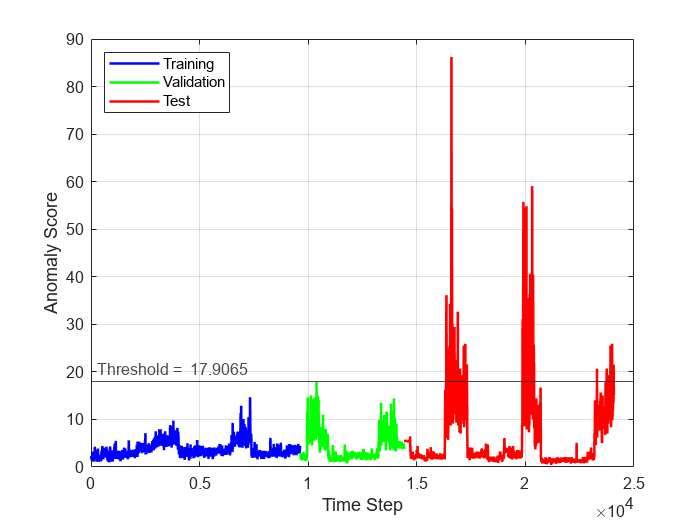
To see the anomaly score for each time step across the entire data set, plot the anomaly scores for the training, validation, and test data against time step. To visualize anomalous time steps, plot a line representing the computed threshold on the same plot. Time steps with anomaly score above the threshold plot correspond to anomalous time steps, whereas time steps with anomaly score below the threshold plot correspond to normal time steps.
numObservationsTrain = numel(scoreTrain);
numObservationsValidation = numel(scoreValidation);
numObservationsTest = numel(scoreTest);
trainTimeIdx = windowSize+(1:numObservationsTrain);
validationTimeIdx = windowSize+trainTimeIdx(end)+(1:numObservationsValidation);
testTimeIdx = windowSize+validationTimeIdx(end)+(1:numObservationsTest);

figure
plot(...
    trainTimeIdx,scoreTrain,'b',...
    validationTimeIdx,scoreValidation,'g',...
    testTimeIdx,scoreTest,'r',...
    'linewidth',1.5)
hold on
yline(threshold,"k-",join(["Threshold = " threshold]),...
    LabelHorizontalAlignment="left");
hold off
xlabel("Time Step")
ylabel("Anomaly Score")
legend("Training","Validation","Test",Location="northwest")
grid on
Detect Anomalies in New Data
featuresNew = feat(numTimeStepsTrain+numTimeStepsValidation+1:end,:);
Obtain the anomaly scores and the channels with the highest anomaly scores in each time step for the data.
featuresNewNormalized = normalize(featuresNew,center=muData,scale=sigmaData);
[XNew,TNew] = processData(featuresNewNormalized,windowSize);
dsXNew = arrayDatastore(XNew,IterationDimension=3);
YNew = modelPredictions(parameters,dsXNew,topKNum);
[scoreNew,channelMaxScores] = deviationScore(YNew,TNew,windowSize);
Obtain the anomaly fraction using the anomaly score and validation threshold.
numObservationsNew = numel(scoreNew);
anomalyFraction = sum(scoreNew>threshold)/numObservationsNew;
Using the channels with the highest anomaly scores in each time step channelMaxScores, compute frequency of anomaly for each channel and visualize the frequency using a bar graph.
anomalousChannels = channelMaxScores(scoreNew>threshold);
for i = 1:numChannels
    frequency(i) = sum(anomalousChannels==i);
end

figure
bar(frequency)
xlabel("Channel")
ylabel("Frequency")
title("Anomalous Node Count")

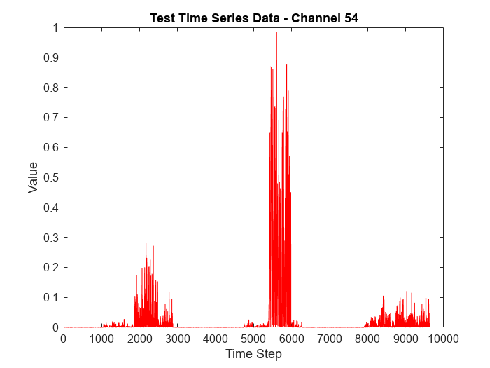
View the channel with the highest anomaly frequency.
[~, channelHighestFrequency] = max(frequency)
channelHighestFrequency = 54
To visualize the time series data corresponding to the channel with the highest anomaly frequency, plot the data values corresponding to the channel against time steps.
figure
plot(featuresNew(:,channelHighestFrequency),'r')
xlabel("Time Step")
ylabel("Value")
title("Test Time Series Data - Channel " + num2str(channelHighestFrequency))
To visualize detected anomalous points in the data corresponding to the channel with highest anomaly frequency
Plot the model predictions and targets corresponding to the channel against time steps to see how the model predictions compare with the targets.
Plot the targets corresponding to the channel at detected anomalous time steps only against detected anomalous time steps to see the anomalous points and compare with how the model predictions compare with the targets.
anomalousTimeSteps = find(scoreNew>threshold);
channelHighestFrequencyTimeSteps = anomalousTimeSteps(anomalousChannels==channelHighestFrequency);

figure
tiledlayout(2,1);
nexttile
plot(1:numObservationsNew,TNew(channelHighestFrequency,:),'r',...
    1:numObservationsNew,YNew(channelHighestFrequency,:),'g')
xlim([1 numObservationsNew])
legend("Targets","Predictions",Location="northwest")
xlabel("Time Step")
ylabel("Normalized Value")
title("Test Data: Channel " + num2str(channelHighestFrequency))
nexttile
plot(channelHighestFrequencyTimeSteps,TNew(channelHighestFrequency,channelHighestFrequencyTimeSteps),'xk')
xlim([1 numObservationsNew])
legend("Anomalous points",Location="northwest")
xlabel("Time Step")
ylabel("Normalized Value")

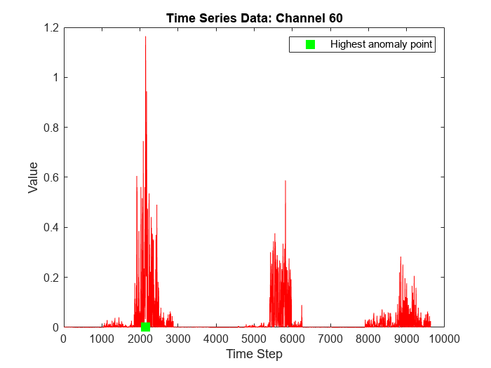
View the channel with the highest anomaly score.
[~,idxMaxScore] = max(scoreNew);
channelHighestAnomalyScore = channelMaxScores(idxMaxScore)
channelHighestAnomalyScore = 60
To visualize the time series data corresponding to the channel with the highest anomaly score, plot the data values corresponding to the channel against time steps and indicate the time step corresponding to the highest anomaly score in the plot.
timeHighestAnomalyScore = idxMaxScore;

figure
plot(featuresNew(:,channelHighestAnomalyScore),'r')
hold on
plot(timeHighestAnomalyScore,0,'s',MarkerSize=10,MarkerEdgeColor='g',MarkerFaceColor='g')
hold off
legend("","Highest anomaly point")
xlabel("Time Step")
ylabel("Value")
title("Time Series Data: Channel " + num2str(channelHighestAnomalyScore))
Process Data Function
The processData function takes as input the features features and the window size windowSize and returns the predictors XData and targets TData for time steps windowSize + 1 to the last time step in features.
function [XData,TData] = processData(features, windowSize)
numObs = size(features,1) - windowSize;
XData = zeros(windowSize,size(features,2),numObs);
for startIndex = 1:numObs
    endIndex = (startIndex-1)+windowSize;
    XData(:,:,startIndex) = features(startIndex:endIndex,:);
end
TData = features(windowSize+1:end,:);
TData = permute(TData,[2 1]);
end
Model Function
The model function, described in the Define Model Function section of the example, takes as input the model parameters parameters, the predictors X, and the top k number topKNum, and returns the predictions and the attention scores obtained from the graphAttention function defined in Graph Attention Function section of the example. The attention scores represent the local weighted adjacency matrix of predicted future values.
function [Y,attentionScores] = model(parameters,X,topKNum)
% Embedding
weights = parameters.embed.weights;
numNodes = size(weights,2) - 1;
embeddingOutput = embed(1:numNodes,weights,DataFormat="CU");

% Graph Structure
adjacency = graphStructure(embeddingOutput,topKNum,numNodes);

% Add self-loop to graph structure
adjacency = adjacency + eye(size(adjacency));

% Graph Attention
embeddingOutput = repmat(embeddingOutput,1,1,size(X,3));
weights = parameters.graphattn.weights;
[outputFeatures,attentionScores] = graphAttention(X,embeddingOutput,adjacency,weights);

% Relu
outputFeatures = relu(outputFeatures);

% Multiply
outputFeatures = embeddingOutput .* outputFeatures;

% Fully Connect
weights = parameters.fc1.weights;
bias = parameters.fc1.bias;
Y = fullyconnect(outputFeatures,weights,bias,DataFormat="UCB");

% Relu
Y = relu(Y);

% Fully Connect
weights = parameters.fc2.weights;
bias = parameters.fc2.bias;
Y = fullyconnect(Y,weights,bias,DataFormat="CB");
end
Model Loss Function
The modelLoss function, described in the Define Model Loss Function of the example, takes as input the model parameters parameters, the predictors X, the targets T, and the top k number topKNum, and returns the loss and the gradients of the loss with respect to the learnable parameters.
function [loss,gradients] = modelLoss(parameters,X,T,topKNum)
Y = model(parameters,X,topKNum);
loss = l2loss(Y,T,DataFormat="CB");
gradients = dlgradient(loss,parameters);
end
Model Predictions Function
The modelPredictions function takes as input the model parameters parameters, the datastore object ds containing the predictors, the top k number topKNum, and optionally the mini-batch size for iterating over mini-batches of read size in the datastore object and returns the model predictions. The function uses a default mini-batch size of 500. However, you can use any value within your hardware memory allowance.
function Y = modelPredictions(parameters,ds,topKNum,minibatchSize)
arguments
    parameters
    ds
    topKNum
    minibatchSize = 500
end

ds.ReadSize = minibatchSize;
Y = [];

reset(ds)
while hasdata(ds)
    data = read(ds);
    data= cat(3,data{:});
    if canUseGPU
        X = gpuArray(dlarray(data));
    else
        X = dlarray(data);
    end
    miniBatchPred = model(parameters,X,topKNum);
    Y = cat(2,Y,miniBatchPred);
end
end
Graph Structure Function
The graphStructure function takes as input channel embedding embedding, top k number topKNum, and the number of channels numChannels, and returns an adjacency matrix representing relations between channels.
The function
Computes a similarity score between channels using cosine similarity.
For each channel, determine related channels from the entire channel set, excluding the channel in consideration, by selecting the
topKNumnumber of channels with the highest similarity score.
function adjacency = graphStructure(embedding,topKNum,numChannels)
% Similarity score
normY = sqrt(sum(embedding.*embedding));
normalizedY = embedding./normY;
score = embedding.' * normalizedY;

% Channel relations
adjacency = zeros(numChannels,numChannels);
for i = 1:numChannels
    topkInd = zeros(1,topKNum);
    scoreNodeI = score(i,:);
    % Make sure that channel i is not in its own candidate set
    scoreNodeI(i) = NaN;
    for j = 1:topKNum
        [~, ind] = max(scoreNodeI);
        topkInd(j) = ind;
        scoreNodeI(ind) = NaN;
    end
    adjacency(i,topkInd) = 1;
end
end
Graph Attention Function
The graphAttention function takes as input the features inputFeatures, channel embedding embedding, learned adjacency matrix adjacency, the learnable parameters weights, and returns learned graph embedding and attention scores.
function [outputFeatures,attentionScore] = graphAttention(inputFeatures,embedding,adjacency,weights)
linearWeights = weights.linear;
attentionWeights = weights.attention;

% Compute linear transformation of input features
value = pagemtimes(linearWeights, inputFeatures);

% Concatenate linear transformation with channel embedding
gate = cat(1,embedding,value);

% Compute attention coefficients
query = pagemtimes(attentionWeights(1, :), gate);
key = pagemtimes(attentionWeights(2, :), gate);

attentionCoefficients = query + permute(key,[2, 1, 3]);
attentionCoefficients = leakyrelu(attentionCoefficients,0.2);

% Compute masked attention coefficients
mask = -10e9 * (1 - adjacency);
attentionCoefficients = (attentionCoefficients .* adjacency) + mask;

% Compute normalized masked attention coefficients
attentionScore = softmax(attentionCoefficients,DataFormat = "UCB");

% Normalize features using normalized masked attention coefficients
outputFeatures = pagemtimes(value, attentionScore);
end
Deviation Score Function
The deviationScore function takes as input the model predictions predictions, the target data targets, the window size windowSize, and returns the deviation score at each time step and the channel that is associated with the deviation score.
The function
Computes an error value between the predictions and targets using
l1loss.Normalizes the error values for each channel by subtracting the median values across time steps from the error values and dividing by the inter-quartile range across time steps.
Obtains the deviation score for each time step as the largest normalized error value across channels.
Finally, computes smoothed deviation score using the moving mean function
movmeanwith a sliding window length ofwindowSize.
function [smoothedScore,channel] = deviationScore(prediction,target,windowSize)
error = l1loss(prediction,target,DataFormat="CB",Reduction="none");
error = gather(double(extractdata(error)));

epsilon=0.01;
normalizedError = (error - median(error,2))./(abs(iqr(error,2)) + epsilon);
[scorePerTime,channel] = max(normalizedError);
smoothedScore = movmean(scorePerTime,windowSize);
end
References
[1] A. Deng and B. Hooi, “Graph neural network-based anomaly detection in multivariate time series,” in Proceedings of the 35th AAAI Conference on Artificial Intelligence, 2021.
See Also
dlarray | dlfeval | dlgradient
Topics
- Custom Loss Functions
- Custom Training Loops
- Custom Training Loop Model Loss Functions
- Sequence Classification Using Deep Learning
- Sequence-to-One Regression Using Deep Learning
- Time Series Forecasting Using Deep Learning
- Initialize Learnable Parameters for Model Function
- Specify Training Options in Custom Training Loop
- List of Functions with dlarray Support