Design Time Series Time-Delay Neural Networks
Begin with the most straightforward dynamic network, which consists of a feedforward network with a tapped delay line at the input. This is called the focused time-delay neural network (FTDNN). This is part of a general class of dynamic networks, called focused networks, in which the dynamics appear only at the input layer of a static multilayer feedforward network. The following figure illustrates a two-layer FTDNN.

This network is well suited to time-series prediction. The following example the use of the FTDNN for predicting a classic time series.
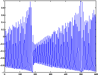
The following figure is a plot of normalized intensity data recorded from a Far-Infrared-Laser in a chaotic state. This is a part of one of several sets of data used for the Santa Fe Time Series Competition [WeGe94]. In the competition, the objective was to use the first 1000 points of the time series to predict the next 100 points. Because our objective is simply to illustrate how to use the FTDNN for prediction, the network is trained here to perform one-step-ahead predictions. (You can use the resulting network for multistep-ahead predictions by feeding the predictions back to the input of the network and continuing to iterate.)

The first step is to load the data, normalize it, and convert it to a time sequence (represented by a cell array):
y = laser_dataset;
y = y(1:600);
Now create the FTDNN network, using the timedelaynet command. This command is similar to the feedforwardnet command, with the additional input of the tapped delay line vector
(the first input). For this example, use a tapped delay line with delays from 1 to 8, and use ten
neurons in the hidden layer:
ftdnn_net = timedelaynet([1:8],10);
ftdnn_net.trainParam.epochs = 1000;
ftdnn_net.divideFcn = '';
Arrange the network inputs and targets for training. Because the network has a tapped delay
line with a maximum delay of 8, begin by predicting the ninth value of the time series. You also
need to load the tapped delay line with the eight initial values of the time series (contained in
the variable Pi):
p = y(9:end);
t = y(9:end);
Pi=y(1:8);
ftdnn_net = train(ftdnn_net,p,t,Pi);
Notice that the input to the network is the same as the target. Because the network has a minimum delay of one time step, this means that you are performing a one-step-ahead prediction.
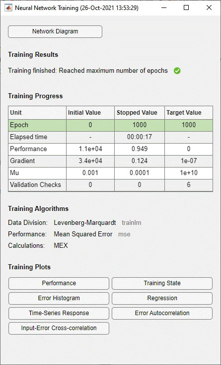
During training, the following training window appears.

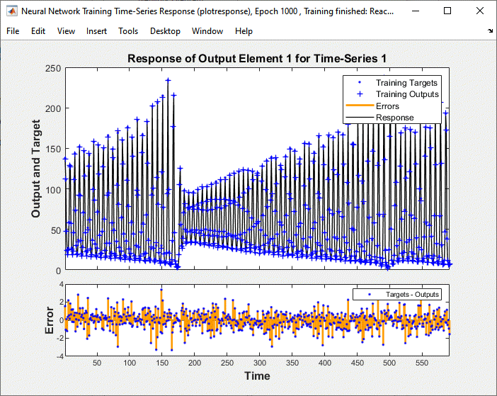
Training stopped because the maximum epoch was reached. From this window, you can display the response of the network by clicking Time-Series Response. The following figure appears.

Now simulate the network and determine the prediction error.
yp = ftdnn_net(p,Pi);
e = gsubtract(yp,t);
rmse = sqrt(mse(e))

rmse =
    0.9740
(Note that gsubtract is a general subtraction function that can
operate on cell arrays.) This result is much better than you could have obtained using a linear
predictor. You can verify this with the following commands, which design a linear filter with the
same tapped delay line input as the previous FTDNN.
lin_net = linearlayer([1:8]);
lin_net.trainFcn='trainlm';
[lin_net,tr] = train(lin_net,p,t,Pi);
lin_yp = lin_net(p,Pi);
lin_e = gsubtract(lin_yp,t);
lin_rmse = sqrt(mse(lin_e))

lin_rmse =
	21.1386
The rms error is 21.1386 for the linear predictor, but 0.9740 for the
nonlinear FTDNN predictor.
One nice feature of the FTDNN is that it does not require dynamic backpropagation to compute the network gradient. This is because the tapped delay line appears only at the input of the network, and contains no feedback loops or adjustable parameters. For this reason, you will find that this network trains faster than other dynamic networks.
If you have an application for a dynamic network, try the linear network first (linearlayer) and then the FTDNN (timedelaynet). If neither network is satisfactory, try one of the more complex
dynamic networks discussed in the remainder of this topic.
Each time a neural network is trained, can result in a different solution due to different initial weight and bias values and different divisions of data into training, validation, and test sets. As a result, different neural networks trained on the same problem can give different outputs for the same input. To ensure that a neural network of good accuracy has been found, retrain several times.
There are several other techniques for improving upon initial solutions if higher accuracy is desired. For more information, see Improve Shallow Neural Network Generalization and Avoid Overfitting.
Prepare Input and Layer Delay States
You will notice in the last section that for dynamic networks there is a significant amount
of data preparation that is required before training or simulating the network. This is because
the tapped delay lines in the network need to be filled with initial conditions, which requires
that part of the original data set be removed and shifted. There is a toolbox function that
facilitates the data preparation for dynamic (time series) networks - preparets. For example, the following lines:
p = y(9:end);
t = y(9:end);
Pi = y(1:8);
can be replaced with
[p,Pi,Ai,t] = preparets(ftdnn_net,y,y);
The preparets function uses the network object to
determine how to fill the tapped delay lines with initial conditions, and how to shift the data
to create the correct inputs and targets to use in training or simulating the network. The
general form for invoking preparets is
[X,Xi,Ai,T,EW,shift] = preparets(net,inputs,targets,feedback,EW)
The input arguments for preparets are the network object
(net), the external (non-feedback) input to the network
(inputs), the non-feedback target (targets), the feedback
target (feedback), and the error weights (EW) (see Train Neural Networks with Error Weights). The difference between external and
feedback signals will become clearer when the NARX network is described in Design Time Series NARX Feedback Neural Networks. For the FTDNN network,
there is no feedback signal.
The return arguments for preparets are the time shift between network inputs
and outputs (shift), the network input for training and simulation
(X), the initial inputs (Xi) for loading the tapped delay
lines for input weights, the initial layer outputs (Ai) for loading the
tapped delay lines for layer weights, the training targets (T), and the error
weights (EW).
Using preparets eliminates the need to manually shift inputs and targets and load tapped delay lines. This is especially useful for more complex networks.