Train Speech Command Recognition Model Using Deep Learning
This example shows how to train a deep learning model that detects the presence of speech commands in audio. The example uses the Speech Commands Dataset [1] to train a convolutional neural network to recognize a set of commands.
To use a pretrained speech command recognition system, see Speech Command Recognition Using Deep Learning (Audio Toolbox).

To run the example quickly, set speedupExample to true. To run the full example as published, set speedupExample to false.
speedupExample =  false;
Set the random seed for reproducibility.
rng defaultLoad Data
This example uses the Google Speech Commands Dataset [1]. Download and unzip the data set.
downloadFolder = matlab.internal.examples.downloadSupportFile("audio","google_speech.zip");
dataFolder = tempdir;
unzip(downloadFolder,dataFolder)
dataset = fullfile(dataFolder,"google_speech");
Augment Data
The network should be able to not only recognize different spoken words but also to detect if the audio input is silence or background noise.
The supporting function, augmentDataset, uses the long audio files in the background folder of the Google Speech Commands Dataset to create one-second segments of background noise. The function creates an equal number of background segments from each background noise file and then splits the segments between the train and validation folders.
augmentDataset(dataset)
Create Training Datastore
Create an audioDatastore (Audio Toolbox) that points to the training data set.
ads = audioDatastore(fullfile(dataset,"train"), ...
    IncludeSubfolders=true, ...
    FileExtensions=".wav", ...
    LabelSource="foldernames");
Specify the words that you want your model to recognize as commands. Label all files that are not commands or background noise as unknown. Labeling words that are not commands as unknown creates a group of words that approximates the distribution of all words other than the commands. The network uses this group to learn the difference between commands and all other words.
To reduce the class imbalance between the known and unknown words and speed up processing, only include a fraction of the unknown words in the training set.
Use subset (Audio Toolbox) to create a datastore that contains only the commands, the background noise, and the subset of unknown words. Count the number of examples belonging to each category.
commands = categorical(["yes","no","up","down","left","right","on","off","stop","go"]);
background = categorical("background");

isCommand = ismember(ads.Labels,commands);
isBackground = ismember(ads.Labels,background);
isUnknown = ~(isCommand|isBackground);

includeFraction = 0.2; % Fraction of unknowns to include.
idx = find(isUnknown);
idx = idx(randperm(numel(idx),round((1-includeFraction)*sum(isUnknown))));
isUnknown(idx) = false;

ads.Labels(isUnknown) = categorical("unknown");

adsTrain = subset(ads,isCommand|isUnknown|isBackground);
adsTrain.Labels = removecats(adsTrain.Labels);
Create Validation Datastore
Create an audioDatastore (Audio Toolbox) that points to the validation data set. Follow the same steps used to create the training datastore.
ads = audioDatastore(fullfile(dataset,"validation"), ...
    IncludeSubfolders=true, ...
    FileExtensions=".wav", ...
    LabelSource="foldernames");

isCommand = ismember(ads.Labels,commands);
isBackground = ismember(ads.Labels,background);
isUnknown = ~(isCommand|isBackground);

includeFraction = 0.2; % Fraction of unknowns to include.
idx = find(isUnknown);
idx = idx(randperm(numel(idx),round((1-includeFraction)*sum(isUnknown))));
isUnknown(idx) = false;

ads.Labels(isUnknown) = categorical("unknown");

adsValidation = subset(ads,isCommand|isUnknown|isBackground);
adsValidation.Labels = removecats(adsValidation.Labels);
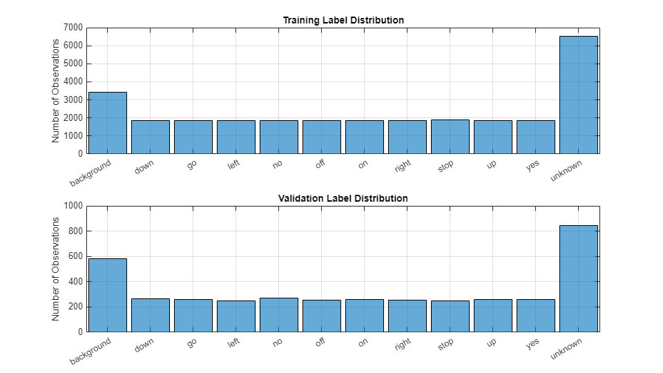
Visualize the training and validation label distributions.
figure(Units="normalized",Position=[0.2,0.2,0.5,0.5])

tiledlayout(2,1)

nexttile
histogram(adsTrain.Labels)
title("Training Label Distribution")
ylabel("Number of Observations")
grid on

nexttile
histogram(adsValidation.Labels)
title("Validation Label Distribution")
ylabel("Number of Observations")
grid on
Speed up the example by reducing the data set, if requested.
if speedupExample
    numUniqueLabels = numel(unique(adsTrain.Labels)); %#ok<UNRCH>
    % Reduce the dataset by a factor of 20
    adsTrain = splitEachLabel(adsTrain,round(numel(adsTrain.Files) / numUniqueLabels / 20));
    adsValidation = splitEachLabel(adsValidation,round(numel(adsValidation.Files) / numUniqueLabels / 20));
end
Prepare Data for Training
To prepare the data for efficient training of a convolutional neural network, convert the speech waveforms to auditory-based spectrograms.
To speed up processing, you can distribute the feature extraction across multiple workers. Start a parallel pool if you have access to Parallel Computing Toolbox™.
if canUseParallelPool && ~speedupExample
    useParallel = true;
    gcp;
else
    useParallel = false;
end
Extract Features
Define the parameters to extract auditory spectrograms from the audio input. segmentDuration is the duration of each speech clip in seconds. frameDuration is the duration of each frame for spectrum calculation. hopDuration is the time step between each spectrum. numBands is the number of filters in the auditory spectrogram.
fs = 16e3; % Known sample rate of the data set.

segmentDuration = 1;
frameDuration = 0.025;
hopDuration = 0.010;

FFTLength = 512;
numBands = 50;

segmentSamples = round(segmentDuration*fs);
frameSamples = round(frameDuration*fs);
hopSamples = round(hopDuration*fs);
overlapSamples = frameSamples - hopSamples;
Create an audioFeatureExtractor (Audio Toolbox) object to perform the feature extraction.
afe = audioFeatureExtractor( ...
    SampleRate=fs, ...
    FFTLength=FFTLength, ...
    Window=hann(frameSamples,"periodic"), ...
    OverlapLength=overlapSamples, ...
    barkSpectrum=true);
setExtractorParameters(afe,"barkSpectrum",NumBands=numBands,WindowNormalization=false);
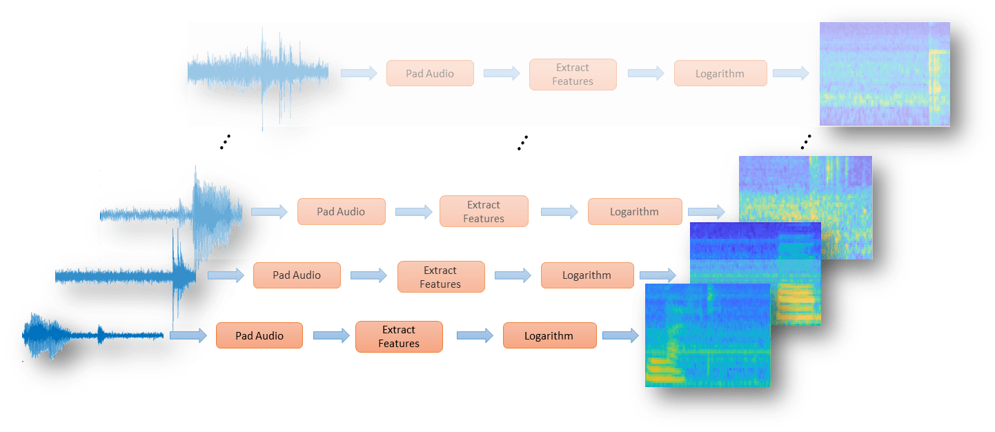
Define a series of transform (Audio Toolbox) on the audioDatastore (Audio Toolbox) to pad the audio to a consistent length, extract the features, and then apply a logarithm.

transform1 = transform(adsTrain,@(x)[zeros(floor((segmentSamples-size(x,1))/2),1);x;zeros(ceil((segmentSamples-size(x,1))/2),1)]);
transform2 = transform(transform1,@(x)extract(afe,x));
transform3 = transform(transform2,@(x){log10(x+1e-6)});
Use the readall (Audio Toolbox) function to read all data from the datastore. As each file is read, it is passed through the transforms before the data is returned.
XTrain = readall(transform3,UseParallel=useParallel);
The output is a numFiles-by-1 cell array. Each element of the cell array corresponds to the auditory spectrogram extracted from a file.
numFiles = numel(XTrain)
numFiles =
28463
[numHops,numBands,numChannels] = size(XTrain{1})numHops = 98
numBands =
50
numChannels =
1
Convert the cell array to a 4-dimensional array with auditory spectrograms along the fourth dimension.
XTrain = cat(4,XTrain{:});

[numHops,numBands,numChannels,numFiles] = size(XTrain)
numHops = 98
numBands =
50
numChannels =
1
numFiles =
28463
Perform the feature extraction steps described above on the validation set.
transform1 = transform(adsValidation,@(x)[zeros(floor((segmentSamples-size(x,1))/2),1);x;zeros(ceil((segmentSamples-size(x,1))/2),1)]);
transform2 = transform(transform1,@(x)extract(afe,x));
transform3 = transform(transform2,@(x){log10(x+1e-6)});
XValidation = readall(transform3,UseParallel=useParallel);
XValidation = cat(4,XValidation{:});
For convenience, isolate the train and validation target labels.
TTrain = adsTrain.Labels;
TValidation = adsValidation.Labels;
Visualize Data
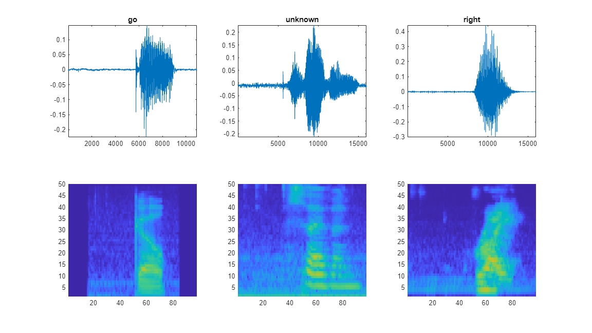
Plot the waveforms and auditory spectrograms of a few training samples. Play the corresponding audio clips.
specMin = min(XTrain,[],"all");
specMax = max(XTrain,[],"all");
idx = randperm(numel(adsTrain.Files),3);
figure(Units="normalized",Position=[0.2,0.2,0.6,0.6]);

tlh = tiledlayout(2,3);
for ii = 1:3
    [x,fs] = audioread(adsTrain.Files{idx(ii)});

    nexttile(tlh,ii)
    plot(x)
    axis tight
    title(string(adsTrain.Labels(idx(ii))))

    nexttile(tlh,ii+3)
    spect = XTrain(:,:,1,idx(ii))';
    pcolor(spect)
    clim([specMin specMax])
    shading flat

    sound(x,fs)
    pause(2)
end
Define Network Architecture
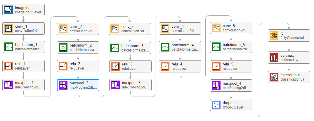
Create a simple network architecture as an array of layers. Use convolutional and batch normalization layers, and downsample the feature maps "spatially" (that is, in time and frequency) using max pooling layers. Add a final max pooling layer that pools the input feature map globally over time. This enforces (approximate) time-translation invariance in the input spectrograms, allowing the network to perform the same classification independent of the exact position of the speech in time. Global pooling also significantly reduces the number of parameters in the final fully connected layer. To reduce the possibility of the network memorizing specific features of the training data, add a small amount of dropout to the input to the last fully connected layer.
The network is small, as it has only five convolutional layers with few filters. numF controls the number of filters in the convolutional layers. To increase the accuracy of the network, try increasing the network depth by adding identical blocks of convolutional, batch normalization, and ReLU layers. You can also try increasing the number of convolutional filters by increasing numF.
To give each class equal total weight in the loss, use class weights that are inversely proportional to the number of training examples in each class. When using the Adam optimizer to train the network, the training algorithm is independent of the overall normalization of the class weights.
classes = categories(TTrain);
classWeights = 1./countcats(TTrain);
classWeights = classWeights'/mean(classWeights);
numClasses = numel(classes);

timePoolSize = ceil(numHops/8);

dropoutProb = 0.2;
numF = 12;
layers = [
    imageInputLayer([numHops,afe.FeatureVectorLength])

    convolution2dLayer(3,numF,Padding="same")
    batchNormalizationLayer
    reluLayer
    maxPooling2dLayer(3,Stride=2,Padding="same")

    convolution2dLayer(3,2*numF,Padding="same")
    batchNormalizationLayer
    reluLayer
    maxPooling2dLayer(3,Stride=2,Padding="same")

    convolution2dLayer(3,4*numF,Padding="same")
    batchNormalizationLayer
    reluLayer
    maxPooling2dLayer(3,Stride=2,Padding="same")

    convolution2dLayer(3,4*numF,Padding="same")
    batchNormalizationLayer
    reluLayer

    convolution2dLayer(3,4*numF,Padding="same")
    batchNormalizationLayer
    reluLayer
    maxPooling2dLayer([timePoolSize,1])
    dropoutLayer(dropoutProb)

    fullyConnectedLayer(numClasses)
    softmaxLayer];
Specify Training Options
To define parameters for training, use trainingOptions. Use the Adam optimizer with a mini-batch size of 128.
miniBatchSize = 128;
validationFrequency = floor(numel(TTrain)/miniBatchSize);
options = trainingOptions("adam", ...
    InitialLearnRate=3e-4, ...
    MaxEpochs=15, ...
    MiniBatchSize=miniBatchSize, ...
    Shuffle="every-epoch", ...
    Plots="training-progress", ...
    Verbose=false, ...
    ValidationData={XValidation,TValidation}, ...
    ValidationFrequency=validationFrequency, ...
    Metrics="accuracy");
Train Network
To train the network, use trainnet. If you do not have a GPU, then training the network can take time.
trainedNet = trainnet(XTrain,TTrain,layers,@(Y,T)crossentropy(Y,T,classWeights(:),WeightsFormat="C"),options);
Evaluate Trained Network
To calculate the final accuracy of the network on the training and validation sets, use minibatchpredict. The network is very accurate on this data set. However, the training, validation, and test data all have similar distributions that do not necessarily reflect real-world environments. This limitation particularly applies to the unknown category, which contains utterances of only a small number of words.
scores = minibatchpredict(trainedNet,XValidation);
YValidation = scores2label(scores,classes,"auto");
validationError = mean(YValidation ~= TValidation);
scores = minibatchpredict(trainedNet,XTrain);
YTrain = scores2label(scores,classes,"auto");
trainError = mean(YTrain ~= TTrain);

disp(["Training error: " + trainError*100 + " %";"Validation error: " + validationError*100 + " %"])
    "Training error: 3.2744 %"
    "Validation error: 6.6217 %"
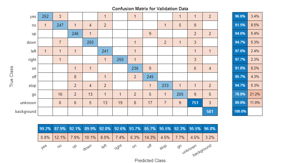
To plot the confusion matrix for the validation set, use confusionchart. Display the precision and recall for each class by using column and row summaries.
figure(Units="normalized",Position=[0.2,0.2,0.5,0.5]);
cm = confusionchart(TValidation,YValidation, ...
    Title="Confusion Matrix for Validation Data", ...
    ColumnSummary="column-normalized",RowSummary="row-normalized");
sortClasses(cm,[commands,"unknown","background"])
When working on applications with constrained hardware resources, such as mobile applications, it is important to consider the limitations on available memory and computational resources. Compute the total size of the network in kilobytes and test its prediction speed when using a CPU. The prediction time is the time for classifying a single input image. If you input multiple images to the network, these can be classified simultaneously, leading to shorter prediction times per image. When classifying streaming audio, however, the single-image prediction time is the most relevant.
for ii = 1:100
    x = randn([numHops,numBands]);
    predictionTimer = tic;
    y = predict(trainedNet,x);
    time(ii) = toc(predictionTimer);
end

disp(["Network size: " + whos("trainedNet").bytes/1024 + " kB"; ...
"Single-image prediction time on CPU: " + mean(time(11:end))*1000 + " ms"])
    "Network size: 310.5391 kB"
    "Single-image prediction time on CPU: 1.8936 ms"
Supporting Functions
Augment Dataset With Background Noise
function augmentDataset(datasetloc)
adsBkg = audioDatastore(fullfile(datasetloc,"background"));
fs = 16e3; % Known sample rate of the data set
segmentDuration = 1;
segmentSamples = round(segmentDuration*fs);

volumeRange = log10([1e-4,1]);

numBkgSegments = 4000;
numBkgFiles = numel(adsBkg.Files);
numSegmentsPerFile = floor(numBkgSegments/numBkgFiles);

fpTrain = fullfile(datasetloc,"train","background");
fpValidation = fullfile(datasetloc,"validation","background");

if ~datasetExists(fpTrain)

    % Create directories
    mkdir(fpTrain)
    mkdir(fpValidation)

    for backgroundFileIndex = 1:numel(adsBkg.Files)
        [bkgFile,fileInfo] = read(adsBkg);
        [~,fn] = fileparts(fileInfo.FileName);

        % Determine starting index of each segment
        segmentStart = randi(size(bkgFile,1)-segmentSamples,numSegmentsPerFile,1);

        % Determine gain of each clip
        gain = 10.^((volumeRange(2)-volumeRange(1))*rand(numSegmentsPerFile,1) + volumeRange(1));

        for segmentIdx = 1:numSegmentsPerFile

            % Isolate the randomly chosen segment of data.
            bkgSegment = bkgFile(segmentStart(segmentIdx):segmentStart(segmentIdx)+segmentSamples-1);

            % Scale the segment by the specified gain.
            bkgSegment = bkgSegment*gain(segmentIdx);

            % Clip the audio between -1 and 1.
            bkgSegment = max(min(bkgSegment,1),-1);

            % Create a file name.
            afn = fn + "_segment" + segmentIdx + ".wav";

            % Randomly assign background segment to either the train or
            % validation set.
            if rand > 0.85 % Assign 15% to validation
                dirToWriteTo = fpValidation;
            else % Assign 85% to train set.
                dirToWriteTo = fpTrain;
            end

            % Write the audio to the file location.
            ffn = fullfile(dirToWriteTo,afn);
            audiowrite(ffn,bkgSegment,fs)

        end

        % Print progress
        fprintf('Progress = %d (%%)\n',round(100*progress(adsBkg)))

    end
end
end
References
[1] Warden P. "Speech Commands: A public dataset for single-word speech recognition", 2017. Available from https://storage.googleapis.com/download.tensorflow.org/data/speech_commands_v0.01.tar.gz. Copyright Google 2017. The Speech Commands Dataset is licensed under the Creative Commons Attribution 4.0 license, available here: https://creativecommons.org/licenses/by/4.0/legalcode.
See Also
trainnet | trainingOptions | dlnetwork | testnet | minibatchpredict | scores2label | analyzeNetwork