Cluster with Self-Organizing Map Neural Network

Self-organizing feature maps (SOFM) learn to classify input vectors according to how they are grouped in the input space. They differ from competitive layers in that neighboring neurons in the self-organizing map learn to recognize neighboring sections of the input space. Thus, self-organizing maps learn both the distribution (as do competitive layers) and topology of the input vectors they are trained on.

The neurons in the layer of an SOFM are arranged originally in physical positions according to a topology function. The function gridtop, hextop, or randtop can arrange the neurons in a grid, hexagonal, or random topology. Distances between neurons are calculated from their positions with a distance function. There are four distance functions, dist, boxdist, linkdist, and mandist. Link distance is the most common. These topology and distance functions are described in Topologies (gridtop, hextop, randtop) and Distance Functions (dist, linkdist, mandist, boxdist).

Here a self-organizing feature map network identifies a winning neuron i* using the same procedure as employed by a competitive layer. However, instead of updating only the winning neuron, all neurons within a certain neighborhood N_i* (d) of the winning neuron are updated, using the Kohonen rule. Specifically, all such neurons i ∊ N_i* (d) are adjusted as follows:

$${}_{i}w(q)={}_{i}w(q-1)+\alpha (p(q)-{}_{i}w(q-1))$$

or

$${}_{i}w(q)=(1-\alpha ){}_{i}w(q-1)+\alpha p(q)$$

Here the neighborhood N_i* (d) contains the indices for all of the neurons that lie within a radius d of the winning neuron i*.

$$N_i(d)=\left\{j,d_{ij}\le d\right\}$$

Thus, when a vector p is presented, the weights of the winning neuron and its close neighbors move toward p. Consequently, after many presentations, neighboring neurons have learned vectors similar to each other.

Another version of SOFM training, called the batch algorithm, presents the whole data set to the network before any weights are updated. The algorithm then determines a winning neuron for each input vector. Each weight vector then moves to the average position of all of the input vectors for which it is a winner, or for which it is in the neighborhood of a winner.

To illustrate the concept of neighborhoods, consider the figure below. The left diagram shows a two-dimensional neighborhood of radius d = 1 around neuron 13. The right diagram shows a neighborhood of radius d = 2.

These neighborhoods could be written as N₁₃(1) = {8, 12, 13, 14, 18} and
N₁₃(2) = {3, 7, 8, 9, 11, 12, 13, 14, 15, 17, 18, 19, 23}.

The neurons in an SOFM do not have to be arranged in a two-dimensional pattern. You can use a one-dimensional arrangement, or three or more dimensions. For a one-dimensional SOFM, a neuron has only two neighbors within a radius of 1 (or a single neighbor if the neuron is at the end of the line). You can also define distance in different ways, for instance, by using rectangular and hexagonal arrangements of neurons and neighborhoods. The performance of the network is not sensitive to the exact shape of the neighborhoods.

Topologies (gridtop, hextop, randtop)

You can specify different topologies for the original neuron locations with the functions gridtop, hextop, and randtop.

The gridtop topology starts with neurons in a rectangular grid similar to that shown in the previous figure. For example, suppose that you want a 2-by-3 array of six neurons. You can get this with

pos = gridtop([2, 3])
pos =
     0     1     0     1     0     1
     0     0     1     1     2     2

Here neuron 1 has the position (0,0), neuron 2 has the position (1,0), and neuron 3 has the position (0,1), etc.

Note that had you asked for a gridtop with the dimension sizes reversed, you would have gotten a slightly different arrangement:

pos = gridtop([3, 2])
pos =
     0     1     2     0     1     2
     0     0     0     1     1     1

You can create an 8-by-10 set of neurons in a gridtop topology with the following code:

pos = gridtop([8 10]);
plotsom(pos)

As shown, the neurons in the gridtop topology do indeed lie on a grid.

The hextop function creates a similar set of neurons, but they are in a hexagonal pattern. A 2-by-3 pattern of hextop neurons is generated as follows:

pos = hextop([2, 3])
pos =
         0    1.0000    0.5000    1.5000         0    1.0000
         0         0    0.8660    0.8660    1.7321    1.7321 

Note that hextop is the default pattern for SOM networks generated with selforgmap.

You can create and plot an 8-by-10 set of neurons in a hextop topology with the following code:

pos = hextop([8 10]);
plotsom(pos)

Note the positions of the neurons in a hexagonal arrangement.

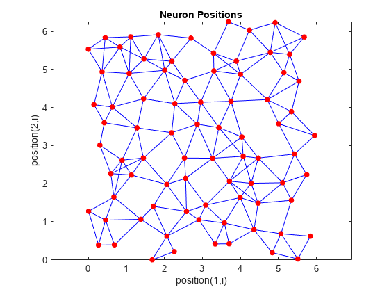
Finally, the randtop function creates neurons in an N-dimensional random pattern. The following code generates a random pattern of neurons.

pos = randtop([2, 3])
pos =
         0    0.7620    0.6268    1.4218    0.0663    0.7862
    0.0925         0    0.4984    0.6007    1.1222    1.4228

You can create and plot an 8-by-10 set of neurons in a randtop topology with the following code:

pos = randtop([8 10]);
plotsom(pos)

For examples, see the help for these topology functions.

Distance Functions (dist, linkdist, mandist, boxdist)

In this toolbox, there are four ways to calculate distances from a particular neuron to its neighbors. Each calculation method is implemented with a special function.

The dist function calculates the Euclidean distances from a home neuron to other neurons. Suppose you have three neurons:

pos2 = [0 1 2; 0 1 2]
pos2 =
     0     1     2
     0     1     2

You find the distance from each neuron to the other with

D2 = dist(pos2)
D2 =
         0    1.4142    2.8284
    1.4142         0    1.4142
    2.8284    1.4142         0

Thus, the distance from neuron 1 to itself is 0, the distance from neuron 1 to neuron 2 is 1.4142, etc.

The graph below shows a home neuron in a two-dimensional (gridtop) layer of neurons. The home neuron has neighborhoods of increasing diameter surrounding it. A neighborhood of diameter 1 includes the home neuron and its immediate neighbors. The neighborhood of diameter 2 includes the diameter 1 neurons and their immediate neighbors.

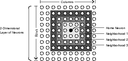
As for the dist function, all the neighborhoods for an S-neuron layer map are represented by an S-by-S matrix of distances. The particular distances shown above (1 in the immediate neighborhood, 2 in neighborhood 2, etc.), are generated by the function boxdist. Suppose that you have six neurons in a gridtop configuration.

pos = gridtop([2, 3])
pos =
     0     1     0     1     0     1
     0     0     1     1     2     2

Then the box distances are

d = boxdist(pos)
d =
     0     1     1     1     2     2
     1     0     1     1     2     2
     1     1     0     1     1     1
     1     1     1     0     1     1
     2     2     1     1     0     1
     2     2     1     1     1     0

The distance from neuron 1 to 2, 3, and 4 is just 1, for they are in the immediate neighborhood. The distance from neuron 1 to both 5 and 6 is 2. The distance from both 3 and 4 to all other neurons is just 1.

The link distance from one neuron is just the number of links, or steps, that must be taken to get to the neuron under consideration. Thus, if you calculate the distances from the same set of neurons with linkdist, you get

dlink =
     0     1     1     2     2     3
     1     0     2     1     3     2
     1     2     0     1     1     2
     2     1     1     0     2     1
     2     3     1     2     0     1
     3     2     2     1     1     0

The Manhattan distance between two vectors x and y is calculated as

D = sum(abs(x-y))

Thus if you have

W1 = [1 2; 3 4; 5 6]
W1 =
     1     2
     3     4
     5     6

and

P1 = [1;1]
P1 =
     1
     1

then you get for the distances

Z1 = mandist(W1,P1)
Z1 =
     1
     5
     9

The distances calculated with mandist do indeed follow the mathematical expression given above.

Architecture

The architecture for this SOFM is shown below.

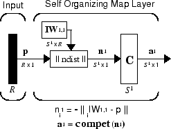
This architecture is like that of a competitive network, except no bias is used here. The competitive transfer function produces a 1 for output element a¹_i corresponding to i*, the winning neuron. All other output elements in a¹ are 0.

Now, however, as described above, neurons close to the winning neuron are updated along with the winning neuron. You can choose from various topologies of neurons. Similarly, you can choose from various distance expressions to calculate neurons that are close to the winning neuron.

Create a Self-Organizing Map Neural Network (selforgmap)

You can create a new SOM network with the function selforgmap. This function defines variables used in two phases of learning:

• Ordering-phase learning rate

• Ordering-phase steps

• Tuning-phase learning rate

• Tuning-phase neighborhood distance

These values are used for training and adapting.

Consider the following example.

Suppose that you want to create a network having input vectors with two elements, and that you want to have six neurons in a hexagonal 2-by-3 network. The code to obtain this network is:

net = selforgmap([2 3]);

Suppose that the vectors to train on are:

P = [.1 .3 1.2 1.1 1.8 1.7 .1 .3 1.2 1.1 1.8 1.7;...
0.2 0.1 0.3 0.1 0.3 0.2 1.8 1.8 1.9 1.9 1.7 1.8];

You can configure the network to input the data and plot all of this with:

net = configure(net,P);
plotsompos(net,P)

The green spots are the training vectors. The initialization for selforgmap spreads the initial weights across the input space. Note that they are initially some distance from the training vectors.

When simulating a network, the negative distances between each neuron’s weight vector and the input vector are calculated (negdist) to get the weighted inputs. The weighted inputs are also the net inputs (netsum). The net inputs compete (compet) so that only the neuron with the most positive net input will output a 1.

Training (learnsomb)

The default learning in a self-organizing feature map occurs in the batch mode (trainbu). The weight learning function for the self-organizing map is learnsomb.

First, the network identifies the winning neuron for each input vector. Each weight vector then moves to the average position of all of the input vectors for which it is a winner or for which it is in the neighborhood of a winner. The distance that defines the size of the neighborhood is altered during training through two phases.

Ordering Phase

This phase lasts for the given number of steps. The neighborhood distance starts at a given initial distance, and decreases to the tuning neighborhood distance (1.0). As the neighborhood distance decreases over this phase, the neurons of the network typically order themselves in the input space with the same topology in which they are ordered physically.

Tuning Phase

This phase lasts for the rest of training or adaption. The neighborhood size has decreased below 1 so only the winning neuron learns for each sample.

Now take a look at some of the specific values commonly used in these networks.

Learning occurs according to the learnsomb learning parameter, shown here with its default value.

Learning Parameter	Default Value	Purpose
LP.init_neighborhood	3	Initial neighborhood size
LP.steps	100	Ordering phase steps

The neighborhood size NS is altered through two phases: an ordering phase and a tuning phase.

The ordering phase lasts as many steps as LP.steps. During this phase, the algorithm adjusts ND from the initial neighborhood size LP.init_neighborhood down to 1. It is during this phase that neuron weights order themselves in the input space consistent with the associated neuron positions.

During the tuning phase, ND is less than 1. During this phase, the weights are expected to spread out relatively evenly over the input space while retaining their topological order found during the ordering phase.

Thus, the neuron's weight vectors initially take large steps all together toward the area of input space where input vectors are occurring. Then as the neighborhood size decreases to 1, the map tends to order itself topologically over the presented input vectors. Once the neighborhood size is 1, the network should be fairly well ordered. The training continues in order to give the neurons time to spread out evenly across the input vectors.

As with competitive layers, the neurons of a self-organizing map will order themselves with approximately equal distances between them if input vectors appear with even probability throughout a section of the input space. If input vectors occur with varying frequency throughout the input space, the feature map layer tends to allocate neurons to an area in proportion to the frequency of input vectors there.

Thus, feature maps, while learning to categorize their input, also learn both the topology and distribution of their input.

You can train the network for 1000 epochs with

net.trainParam.epochs = 1000;
net = train(net,P);

plotsompos(net,P)

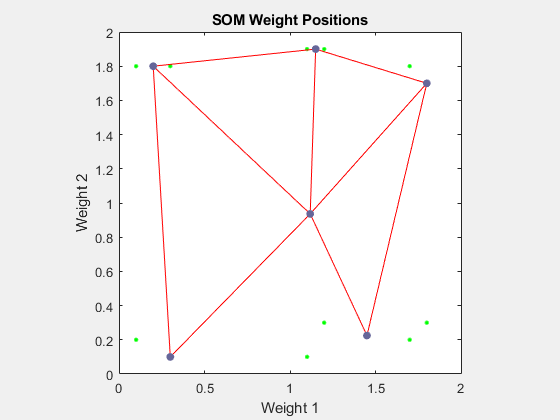
You can see that the neurons have started to move toward the various training groups. Additional training is required to get the neurons closer to the various groups.

As noted previously, self-organizing maps differ from conventional competitive learning in terms of which neurons get their weights updated. Instead of updating only the winner, feature maps update the weights of the winner and its neighbors. The result is that neighboring neurons tend to have similar weight vectors and to be responsive to similar input vectors.

Examples

Two examples are described briefly below. You also might try the similar examples One-Dimensional Self-Organizing Map and Two-Dimensional Self-Organizing Map.

One-Dimensional Self-Organizing Map

Consider 100 two-element unit input vectors spread evenly between 0° and 90°.

angles = 0:0.5*pi/99:0.5*pi;

Here is a plot of the data.

P = [sin(angles); cos(angles)];

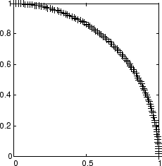
A self-organizing map is defined as a one-dimensional layer of 10 neurons. This map is to be trained on these input vectors shown above. Originally these neurons are at the center of the figure.

Of course, because all the weight vectors start in the middle of the input vector space, all you see now is a single circle.

As training starts the weight vectors move together toward the input vectors. They also become ordered as the neighborhood size decreases. Finally the layer adjusts its weights so that each neuron responds strongly to a region of the input space occupied by input vectors. The placement of neighboring neuron weight vectors also reflects the topology of the input vectors.

Note that self-organizing maps are trained with input vectors in a random order, so starting with the same initial vectors does not guarantee identical training results.

Two-Dimensional Self-Organizing Map

This example shows how a two-dimensional self-organizing map can be trained.

First some random input data is created with the following code:

P = rands(2,1000);

Here is a plot of these 1000 input vectors.

A 5-by-6 two-dimensional map of 30 neurons is used to classify these input vectors. The two-dimensional map is five neurons by six neurons, with distances calculated according to the Manhattan distance neighborhood function mandist.

The map is then trained for 5000 presentation cycles, with displays every 20 cycles.

Here is what the self-organizing map looks like after 40 cycles.

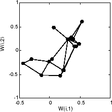
The weight vectors, shown with circles, are almost randomly placed. However, even after only 40 presentation cycles, neighboring neurons, connected by lines, have weight vectors close together.

Here is the map after 120 cycles.

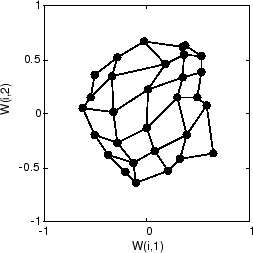
After 120 cycles, the map has begun to organize itself according to the topology of the input space, which constrains input vectors.

The following plot, after 500 cycles, shows the map more evenly distributed across the input space.

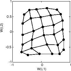
Finally, after 5000 cycles, the map is rather evenly spread across the input space. In addition, the neurons are very evenly spaced, reflecting the even distribution of input vectors in this problem.

Thus a two-dimensional self-organizing map has learned the topology of its inputs' space.

It is important to note that while a self-organizing map does not take long to organize itself so that neighboring neurons recognize similar inputs, it can take a long time for the map to finally arrange itself according to the distribution of input vectors.

Training with the Batch Algorithm

The batch training algorithm is generally much faster than the incremental algorithm, and it is the default algorithm for SOFM training. You can experiment with this algorithm on a simple data set with the following commands:

x = simplecluster_dataset
net = selforgmap([6 6]);
net = train(net,x);

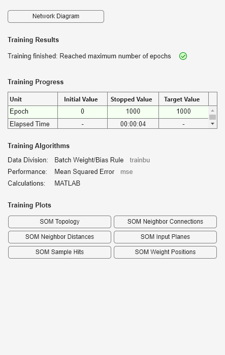
This command sequence creates and trains a 6-by-6 two-dimensional map of 36 neurons. During training, the following figure appears.

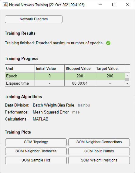
There are several useful visualizations that you can access from this window. If you click SOM Weight Positions, the following figure appears, which shows the locations of the data points and the weight vectors. As the figure indicates, after only 200 iterations of the batch algorithm, the map is well distributed through the input space.

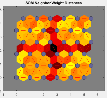
When the input space is high dimensional, you cannot visualize all the weights at the same time. In this case, click SOM Neighbor Distances. The following figure appears, which indicates the distances between neighboring neurons.

This figure uses the following color coding:

• The blue hexagons represent the neurons.

• The red lines connect neighboring neurons.

• The colors in the regions containing the red lines indicate the distances between neurons.

• The darker colors represent larger distances.

• The lighter colors represent smaller distances.

Four groups of light segments appear, bounded by some darker segments. This grouping indicates that the network has clustered the data into four groups. These four groups can be seen in the previous weight position figure.

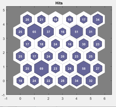
Another useful figure can tell you how many data points are associated with each neuron. Click SOM Sample Hits to see the following figure. It is best if the data are fairly evenly distributed across the neurons. In this example, the data are concentrated a little more in the corner neurons, but overall the distribution is fairly even.

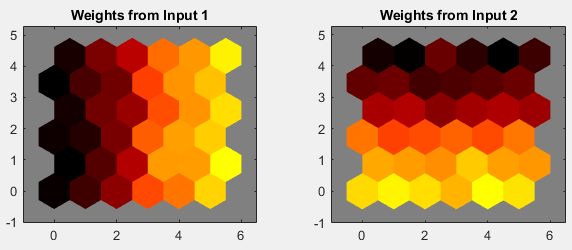
You can also visualize the weights themselves using the weight plane figure. Click SOM Input Planes in the training window to obtain the next figure. There is a weight plane for each element of the input vector (two, in this case). They are visualizations of the weights that connect each input to each of the neurons. (Lighter and darker colors represent larger and smaller weights, respectively.) If the connection patterns of two inputs are very similar, you can assume that the inputs were highly correlated. In this case, input 1 has connections that are very different than those of input 2.

You can also produce all of the previous figures from the command line. Try these plotting commands: plotsomhits, plotsomnc, plotsomnd, plotsomplanes, plotsompos, and plotsomtop.