csape

Cubic spline interpolation with end conditions

Syntax

pp = csape(x,y)

pp = csape(x,y,conds)

pp = csape(x,[e1,y,e2],conds)

pp = csape({x1,...,xn},___)

Description

pp = csape(x,y) returns the cubic spline interpolation to the given data (x,y) in ppform form. The function applies Lagrange end conditions to each end of the data, and matches the spline endslopes to the slope of the cubic polynomial that fits the last four data points at each end. Data values at the same site are averaged.

pp = csape(x,y,conds) uses the end conditions specified by conds.

pp = csape(x,[e1,y,e2],conds) uses the end conditions specified by conds and the values e1 and e2 for the left and right end condition values, respectively.

pp = csape({x1,...,xn},___) returns the cubic spline interpolation for gridded data using the univariate mesh inputs x1,...,xn. In this case, y is an n+r-dimensional array, where r is the dimensionality of each data value. conds is a cell array with n entries, which provides end conditions for each of the n variables. In some cases, you must supply end conditions for end conditions. You can use this syntax with any of the arguments in the previous syntaxes.

Examples

Use Customized End Conditions with csape

You can implement custom end conditions using the csape function. Suppose you want to enforce the following condition at the leftmost endpoint, $\mathit{e}=$x(1)

$$\lambda (s)\equiv aDs(e)+b{D}^{2}s(e)=c$$

for the given scalars $\mathit{a}$,$\mathit{b}$, and $\mathit{c}$. You can compute the cubic spine interpolation $\mathit{s}$ as the sum of $$s_1$$ (the cubic spine interpolation of the given data using the default end conditions) and $$s_0$$ (the cubic spine interpolation of zero data using some nontrivial end conditions):

$$s=s_1+\frac{c-\lambda (s_1)}{\lambda (s_0)}{s}_0$$

The end conditions you specify in $$s_0$$ do not have to be the final desired end conditions $$\lambda (s)$$.

This example uses the titanium test data, a standard data set used in data fitting. Load the data using the titanium function.

[x,y] = titanium;

Define the coefficients for $$\lambda (s)$$.

a = -2;
b = -1;
c = 0;

The end condition applies to the leftmost end of the data set.

e = x(1);

Now, calculate the cubic spline interpolation of the data set without imposing the end conditions.

s1 = csape(x,y);

To calculate $$s_0$$, use zero data of the same length as y with an additional set of nontrivial end conditions.

yZero = zeros(1,length(y));

The 1-by-2 matrix conds sets the end conditions by specifying the spline derivatives to fix. This example uses end conditions only on the left end of the data, so use conds to fix the first derivative at the left end. At the right end, fix the value of the function itself.

conds = [1 0];

To specify the values to fix the function or its derivatives to, add them as additional values to the data set for fitting - in this case, yZero. The first element specifies the value at the left end, while the last element specifies the value at for the right end.

At the left end, fix the first derivative of the spline to have a value of 1. At the right end, fix the function itself to be 0 (the original value of the final element of yZero). Concatenate these end condition values at the respective ends of yZero and use csape to find the spline that fits the data with these end condition values.

s0 = csape(x,[1 yZero 0],conds);

Calculate the fully fitted spline from that data by using the aforementioned expression for $\mathit{s}$. To do this, calculate the values for $${\lambda }_0=\lambda (s_0)$$ and $${\lambda }_1=\lambda (s_1)$$ using the first and second derivatives of the splines $$s_0$$ and $$s_1$$.

d1s1 = fnder(fnbrk(s1,1));
d2s1 = fnder(d1s1);
d1s0 = fnder(fnbrk(s0,1));
d2s0 = fnder(d1s0);

Calculate the derivatives of the first polynomial piece of the spline, as the end conditions apply to the left end of the data only.

lam1 = a*fnval(d1s1, e) + b*fnval(d2s1,e);
lam0 = a*fnval(d1s0, e) + b*fnval(d2s0,e);

Now use $${\lambda }_1$$ and $${\lambda }_0$$ to calculate the final, fully fitted spline.

pp = fncmb(s0,(c-lam1)/lam0,s1);

Plot the spline to compare the results of the default fit and the end conditions.

fnplt(pp,[594, 632])
hold on
fnplt(s1,'b--',[594, 632])
plot(x,y,'ro','MarkerFaceColor','r')
hold off
axis([594, 632, 0.62, 0.655])
legend 'Desired end conditions' ...
'Default end-conditions' 'Data' ...
    Location SouthEast

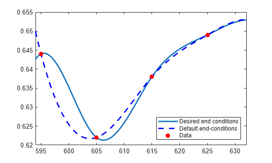
The stationary point near the first data point shows that the end conditions are implemented in the fit.

Fit Multivariate Data

Use csape to fit multivariate, vector-valued data. This example fits vector-valued data using different end conditions for each independent variable.

First, define the data. For this example, define the 3-dimensional vectors v over a 2-dimensional field, with clamped conditions or prescribed slopes in the x direction and periodic end conditions in the y direction.

x = 0:4;
y = -2:2;

s2 = 1/sqrt(2);

v = zeros( 3, 7, 5 );
v(1,:,:) = [1 0 s2 1 s2 0 -1].'*[1 0 -1 0 1];
v(2,:,:) = [1 0 s2 1 s2 0 -1].'*[0 1 0 -1 0];
v(3,:,:) = [0 1 s2 0 -s2 -1 0].'*[1 1 1 1 1];

v is a 3-dimensional array with v(:,i+1,j) as the vector value at coordinate x(i),y(j). Two additional entries in the x dimension specify the slope values: the data points v(:,1,j) and v(:,7,j) provide the value of the first derivative along the lines x = 0 and x = 4 for the clamped end conditions. In the y dimension, the periodic end conditions do not require any additional specification.

Now, calculate the multivariate cubic spline interpolation using csape.

sph = csape({x,y},v,{'clamped','periodic'});

To plot the result, first evaluate the spline over a suitable interval.

values = fnval(sph,{0:.1:4,-2:.1:2});

surf(squeeze(values(1,:,:)), ...
squeeze(values(2,:,:)), squeeze(values(3,:,:)));

axis equal
axis off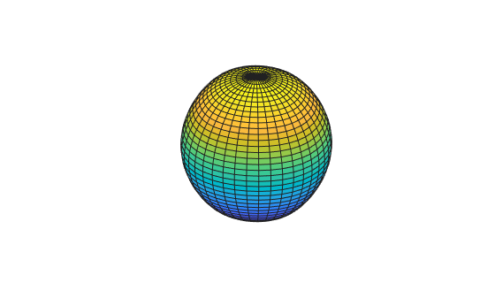

You can also evaluate and plot the spline surface using the simple command fnplt(sph). Note that v is a 3-dimensional array, and v(:,i+1,j) is the 3-vector to match at (x(i),y(j)), i=1:5, j=1:5. Additionally, in accordance with conds{1} being 'clamped', size(v,2) is 7 (and not 5), and the first and last entry of v(r,:,j) specify the end slope values.

Supply End Conditions for End Conditions

In some cases, you must supply end conditions of end conditions. In this bivariate example, you reproduce the bicubic polynomial g(x,y) = x³y³ by complete bicubic interpolation. You then derive the needed data, including end condition values, directly from g to make it easier to see how the end condition values must be placed. Finally, you check the result.

sites = {[0 1],[0 2]}; coefs = zeros(4, 4); coefs(1,1) = 1;
g = ppmak(sites,coefs);
Dxg = fnval(fnder(g,[1 0]),sites);
Dyg = fnval(fnder(g,[0 1]),sites);
Dxyg = fnval(fnder(g,[1 1]),sites);

f = csape(sites,[Dxyg(1,1),   Dxg(1,:),    Dxyg(1,2); ...
                 Dyg(:,1), fnval(g,sites), Dyg(:,2) ; ...
                 Dxyg(2,1),   Dxg(2,:),    Dxyg(2,2)], ...
                                          {'complete','complete'});
if any(squeeze(fnbrk(f,'c'))-coefs)
    disp( 'this is wrong' )
end

Input Arguments

x — Data sites

vector | cell array

Data sites of data values y to fit, specified as a vector or as a cell array for multivariate data. The function creates spline s knots at each data site x such that s(x(j)) = y(:,j) for all j.

For multivariate, gridded data, specify x as a cell array that provides the data site in each variable dimension, such that s(x1(i),x2(j),...,xn(k)) = y(:,i,j,...,k).

Data Types: single | double

y — Data values to fit

vector | matrix | array

Data values to fit during creation of the spline, specified as a vector, matrix, or array. You can specify the data values y(:,j) as scalars, matrices, or n-dimensional arrays. Data values given at the same data site x are averaged.

Data Types: single | double

conds — End conditions

'clamped' | 'complete' | 'not-a-knot' | 'periodic' | 'second' | 'variational' | 1-by-2 matrix

End conditions for the spline, specified as 'complete' or 'clamped', 'not-a-knot', 'periodic', 'second', 'variational', or as a 1-by-2 matrix. The predefined options for conds impose identical end conditions at each end of the data. You can specify different end conditions at each end by supplying conds as a 1-by-2 matrix.

The available predefined end conditions are as follows.

'complete' or 'clamped'	Match the endslopes to the given values e1 and e2. If you do not provide values for e1 and e2, this option matches the default Lagrangian end conditions.
'not-a-knot'	Make the second and second-last sites inactive knots. This option ignores any values you provide for e1 and e2.
'periodic'	Match the first and second derivatives at the left end with those at the right end.
'second'	Match the end second derivatives to the given values e1 and e2. If you do not provide values e1 and e2, this option uses the default value of 0 for both. With the default values, this option is the same as 'variational'.
'variational'	Set the end second derivatives equal to zero. This option ignores any values you provide for e1 and e2.

To specify different end conditions at each end, supply conds as a 1-by-2 matrix. The elements of this matrix elements specify the order of the spline derivative fixed by the end conditions. Setting conds(j) = i fixes the ith derivative Dⁱs to an end condition value.

The default end condition value is the derivative of the cubic interpolant at the left four sites when conds(1) = 1 and is 0 otherwise. Set end condition values for the left and right sides of the data by specifying e1 and e2, respectively.

You can specify the value of conds(j) as 0, 1, or 2. If you specify a different value or do not specify conds(j), then conds(j) is 1 and the corresponding end condition value is the default value.

The following pre-defined end conditions are available.

clamped	Ds(e) = ej	if conds(j) == 1
curved	D2s(e) = ej	if conds(j) == 2
periodic	Drs(a) = Drs(b), r = 1,2	if conds == [0 0]
variational	D2s(e) = 0	if conds(j) == 2 & ej == 0

e, a, and b refer to the left or right data locations; ej is e1 for the left end of the data and e2 for the right end of the data.

You can supply the optional end condition values e1 and e2 whether you use predefined or user-defined options for conds. However, note that some predefined options for conds ignore any end condition values you provide.

Example: 'clamped', [1 0]

e1 — Left end condition value

scalar

Left end condition value for the spline, specified as a scalar value. e1 specifies the value for the ith derivative at the left end of the data, where conds provides i. Even if you use different end conditions at the two ends, if you supply an end condition value at one end you must also supply one for the other end.

Note that some predefined options for conds ignore any end condition values you provide.

The default value for e1 is the derivative of the cubic interpolant at the left four sites when conds(1) = 1 and is 0 otherwise.

Data Types: single | double

e2 — Right end condition value

scalar

Right end condition value for the spline, specified as a scalar value. e2 specifies the value for the ith derivative at the right end of the data, where conds provides i. Even if you use different end conditions at the two ends, if you supply an end condition value at one end you must also supply one for the other end.

Note that some predefined options for conds ignore any end condition values you provide.

The default value for e2 is the derivative of the cubic interpolant at the right four sites when conds(2) = 1 and is 0 otherwise.

Data Types: single | double

Output Arguments

pp — Spline in ppform

spline structure

Spline in ppform, returned as a structure with these fields.

Form — Form of spline

pp

Form of the spline, returned as pp. pp indicates that the spline is given in piecewise polynomial form.

Breaks — Knot locations of spline

vector | cell array

Knot positions of the spline, returned as a vector or as a cell array of vectors for multivariate data. Vectors contain strictly increasing elements that represent the start and end of each of the intervals over which the polynomial pieces are defined.

Coefs — Coefficients of polynomials

matrix | array

Coefficients of polynomials for each piece, returned as a matrix or as an array for multivariate data.

Pieces — Number of polynomial pieces

scalar | vector

Number of polynomial pieces describing the spline, returned as a scalar or as a vector of numbers of pieces in each variable for multivariate data.

Order — Order of polynomials

scalar | vector

Order of the polynomial function describing each polynomial piece of the spline, returned as a scalar or as a vector containing the order in each variable for multivariate data.

Dim — Dimensionality

scalar

Dimensionality of the target function, returned as a scalar.

Algorithms

The relevant tridiagonal linear system is constructed and solved using the sparse matrix capabilities of MATLAB^®.

The csape command calls on a much expanded version of the Fortran routine CUBSPL in PGS.