PID Controller Design at the Command Line

This example shows how to design a PID controller for the plant given by:

$s y s = \frac{1}{{(s + 1)}^{3}} .$

As a first pass, create a model of the plant and design a simple PI controller for it.

sys = zpk([],[-1 -1 -1],1); 
[C_pi,info] = pidtune(sys,'PI')

C_pi =
 
             1 
  Kp + Ki * ---
             s 

  with Kp = 1.14, Ki = 0.454
 
Continuous-time PI controller in parallel form.
Model Properties

info = struct with fields:
                Stable: 1
    CrossoverFrequency: 0.5205
           PhaseMargin: 60.0000

C_pi is a pid controller object that represents a PI controller. The fields of info show that the tuning algorithm chooses an open-loop crossover frequency of about 0.52 rad/s.

Examine the closed-loop step response (reference tracking) of the controlled system.

T_pi = feedback(C_pi*sys, 1);
step(T_pi)

MATLAB figure

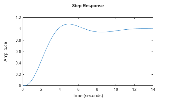
To improve the response time, you can set a higher target crossover frequency than the result that pidtune automatically selects, 0.52. Increase the crossover frequency to 1.0.

[C_pi_fast,info] = pidtune(sys,'PI',1.0)

C_pi_fast =
 
             1 
  Kp + Ki * ---
             s 

  with Kp = 2.83, Ki = 0.0495
 
Continuous-time PI controller in parallel form.
Model Properties

info = struct with fields:
                Stable: 1
    CrossoverFrequency: 1
           PhaseMargin: 43.9973

The new controller achieves the higher crossover frequency, but at the cost of a reduced phase margin.

Compare the closed-loop step response with the two controllers.

T_pi_fast = feedback(C_pi_fast*sys,1);
step(T_pi,T_pi_fast)

MATLAB figure

axis([0 30 0 1.4])

legend('PI','PI,fast')

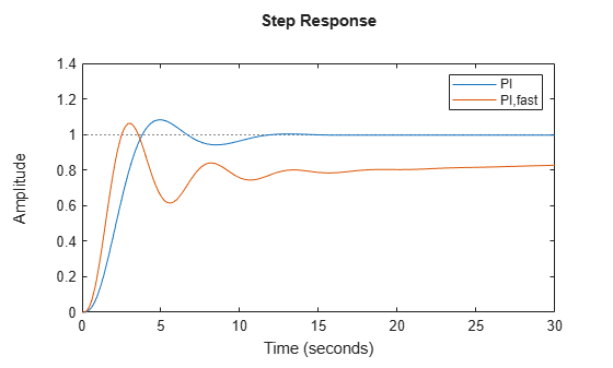
This reduction in performance results because the PI controller does not have enough degrees of freedom to achieve a good phase margin at a crossover frequency of 1.0 rad/s. Adding a derivative action improves the response.

Design a PIDF controller for Gc with the target crossover frequency of 1.0 rad/s.

[C_pidf_fast,info] = pidtune(sys,'PIDF',1.0)

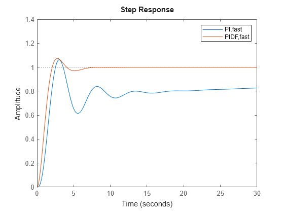
The fields of info show that the derivative action in the controller allows the tuning algorithm to design a more aggressive controller that achieves the target crossover frequency with a good phase margin.

Compare the closed-loop step response and disturbance rejection for the fast PI and PIDF controllers.

T_pidf_fast =  feedback(C_pidf_fast*sys,1);
step(T_pi_fast, T_pidf_fast);
axis([0 30 0 1.4]);
legend('PI,fast','PIDF,fast');

You can compare the input (load) disturbance rejection of the controlled system with the fast PI and PIDF controllers. To do so, plot the response of the closed-loop transfer function from the plant input to the plant output.

S_pi_fast = feedback(sys,C_pi_fast);
S_pidf_fast = feedback(sys,C_pidf_fast);
step(S_pi_fast,S_pidf_fast);
axis([0 50 0 0.4]);
legend('PI,fast','PIDF,fast');

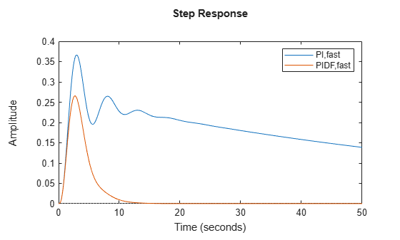
This plot shows that the PIDF controller also provides faster disturbance rejection.

PID Controller Design at the Command Line

See Also

Topics