LPV Model of Magnetic Levitation System

This example uses an analytic linear parameter-varying (LPV) model of a magnetic levitation system to control the height of a ball. In this example, you build the LPV plant model directly from the linearized equations of motion.

Nonlinear System

This figure shows the magnetic ball levitation device and its key components. A current $\mathit{i}$ (A) is supplied to a coil, which creates a magnetic force on the ball. The position of the ball is denoted by $\mathit{h}$ (m). An infrared sensor measures the position of the ball $\mathit{y}$ (V). The objective is to make the ball levitate at a desired position $\bar{\mathit{h}}$. There are two key forces on the ball: the gravity pull ${\mathit{F}}_{\mathit{g}}$ and magnetic force ${\mathit{F}}_{\mathit{m}}$.

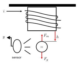
This nonlinear equation defines the dynamics of the model.

$${\mathit{m}}_{\mathit{b}}\ddot{\mathit{h}}={\mathit{m}}_{\mathit{b}}\mathit{g}-\alpha \frac{{\mathit{i}\left(\mathit{t}\right)}^2}{{\mathit{h}\left(\mathit{t}\right)}^2}$$

Here:

• ${\mathit{m}}_{\mathit{b}}$ is the mass of the ball (kg).

• $\mathit{g}$ is the gravitational acceleration (m/s^2).

• $\alpha$ is the magnetic force constant (N$\times$m/(A^2)).

Define the model parameters.

mb = 0.02;
g = 9.81;
alpha = 2.4832e-5;

Equilibrium Conditions

An equilibrium (steady-state) condition with ball height $\bar{\mathit{h}}$ is characterized by the equation

$$0={\mathit{m}}_{\mathit{b}}\mathit{g}-\alpha \frac{{\bar{\mathit{i}}}^2}{{\bar{\mathit{h}}}^2}$$

The required current to maintain this height is

$$\bar{\mathit{i}}=\sqrt{\frac{{\mathit{m}}_{\mathit{b}}\mathit{g}}{\alpha }}\bar{\mathit{h}}$$

Linearized Equations of Motion

To build an LPV approximation of this plant, choose $\mathit{p}=\bar{\mathit{h}}$ as scheduling variable and linearize the equations of motion around the $\mathit{p}$-dependent equilibrium conditions

$${\mathit{x}}_0\left(\mathit{p}\right)=\left(\begin{array}{c}\bar{\mathit{h}}\\ 0\end{array}\right),{\mathit{u}}_0\left(\mathit{p}\right)=\bar{\mathit{i}}=\sqrt{\frac{{\mathit{m}}_{\mathit{b}}\mathit{g}}{\alpha }}\bar{\mathit{h}},{\mathit{y}}_0\left(\mathit{p}\right)=\bar{\mathit{h}}$$

This yields the LPV model

$$\dot{\mathit{x}}=\mathit{A}\left(\mathit{p}\right)\left(\mathit{x}-{\mathit{x}}_0\left(\mathit{p}\right)\right)+\mathit{B}\left(\mathit{p}\right)\left(\mathit{u}-{\mathit{u}}_0\left(\mathit{p}\right)\right)$$

$\mathit{y}={\mathit{y}}_0\left(\mathit{p}\right)+\mathit{C}\left(\mathit{x}-{\mathit{x}}_0\left(\mathit{p}\right)\right)$

with

$$\mathit{x}=\left(\begin{array}{c}\mathit{h}\\ \dot{\mathit{h}}\end{array}\right),\mathit{u}=\mathit{i},\mathit{y}=\mathit{h},\mathit{A}=\left(\begin{array}{cc}0& 1\\ {\mathit{a}}_0\left(\mathit{p}\right)& 0\end{array}\right),\mathit{B}=\left(\begin{array}{c}0\\ {\mathit{b}}_0\left(\mathit{p}\right)\end{array}\right),\mathit{C}=\left(\begin{array}{cc}1& 0\end{array}\right)$$

and

$${\mathit{a}}_0\left(\mathit{p}\right)=\frac{2\mathit{g}}{\mathit{p}},{\mathit{b}}_0\left(\mathit{p}\right)=-2\frac{\sqrt{\mathit{g}\alpha /{\mathit{m}}_{\mathit{b}}}}{\mathit{p}}$$

The matrices and offsets of this system are defined in the function dataFcnMaglev.m.

Use lpvss to create the model.

Glpv = lpvss('h',@dataFcnMaglev);

Gain-Scheduled PID Controller

For PID tuning, pick a few values of $\mathit{h}$ and sample the LPV dynamics at these heights to obtain local LTI models.

Pick three height values between 0.05 and 0.25.

hmin = 0.05;
hmax = 0.25;
hcd = linspace(hmin,hmax,3);
[Ga,Goffsets] = sample(Glpv,[],hcd);
size(Ga)

1x3 array of state-space models.
Each model has 1 outputs, 1 inputs, and 2 states.

Use pidtune to tune a PID controller for each value of $\mathit{h}$. The target crossover frequency is set to 50 rad/s.

wc = 50;
Ka = pidtune(Ga,'pid',wc);
Ka.Tf = 0.001;

Now use ssInterpolant to construct a gain-scheduled PID controller that linearly interpolates the tuned gains between the selected values of $\mathit{h}$. This controller also uses the trim current ${\mathit{u}}_0\left(\mathit{p}\right)$ as feedforward control so that the PID regulates the current around its equilibrium value.

Ka.SamplingGrid.h = hcd;
Koffsets = struct('y',{Goffsets.u});
Klpv = ssInterpolant(ss(Ka),Koffsets);

LTI Analysis

For evaluation purpose, model the ideal response as a second-order systems Tideal.

wn = 30;
zeta = 0.7;
Tideal = tf(wn^2,[1 2*zeta*wn wn^2]);

Sample the closed-loop LPV dynamics over a finer $\mathit{h}$ grid.

hs = linspace(hmin,hmax,5);

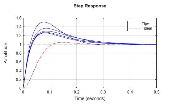
Simulate the step response of the closed-loop model and compare with Tideal.

Tlpv = feedback(Glpv*Klpv,1);
step(sample(Tlpv,[],hs),'b',Tideal,'r--',0.5);
grid on
legend('Tlpv','Tideal')

The closed-loop system has additional zeros not in the ideal response Tideal. These zeros arise from the PID controller and cause a shorter rise time and larger overshoot.

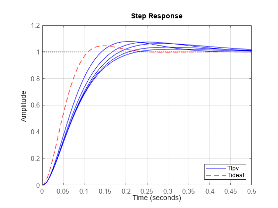
You can use a two degree-of-freedom architecture with a reference prefilter Fref to reduce the overshoot. Model the prefilter as an LTI system for simplicity.

Fref = ss(-10,10,1,0);
step(sample(Tlpv*Fref,[],hs),'b',Tideal,'r--',0.5);
grid on;
legend('Tlpv','Tideal','Location','Southeast');

LPV Simulations

To approximate the nonlinear closed-loop response, simulate the transient response of the closed-loop LPV model with a pre-filter. This requires you to specify the parameter trajectory $\mathit{p}\left(\mathit{t}\right)=\mathit{h}\left(\mathit{t}\right)$, which is not known beforehand. As a proxy, you can set to the ideal response produced by Tideal*Fref.

CL = Tlpv*Fref;

Set the initial height and step signal parameters.

h0 = (hmin+hmax)/2;
tstep = 0.2;  Tf = 1.2;  hStepAmp = 0.25*h0;

Set $\mathit{p}\left(\mathit{t}\right)$ to ideal trajectory and simulate the response.

t = linspace(0,tstep+Tf,100);
StepConfig = RespConfig('InputOffset',h0,'Delay',tstep,'Amplitude',hStepAmp);
p_ideal = step(Tideal*Fref,t,StepConfig);
y1 = step(CL,t,p_ideal,StepConfig);

Alternatively, to use the true trajectory, you can specify $\mathit{p}\left(\mathit{t}\right)$ implicitly as a function $\mathit{F}\left(\mathit{t},\mathit{x},\mathit{u}\right)$ of time $\mathit{t}$, input $\mathit{u}$, and state $\mathit{x}$. Here $\mathit{p}\left(\mathit{t}\right)$ is just the first state.

Set $\mathit{p}\left(\mathit{t}\right)=\mathit{h}\left(\mathit{t}\right)$ and simulate the step response.

pFcn = @(t,x,u) x(1);
StepConfig = RespConfig('InputOffset',h0,'Delay',tstep,...
   'Amplitude',hStepAmp,'InitialParameter',h0);
y2 = step(CL,t,pFcn,StepConfig);

Plot and compare the two responses.

plot(t,y1,t,y2);
legend('p ideal','p true','Location','Southeast');
grid

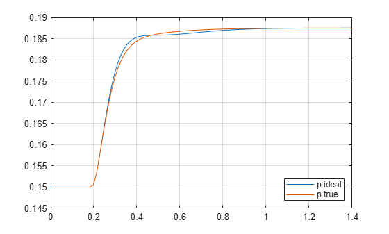
The two responses are close to each other. The Simulink-based counterpart of this example shows that the nonlinear response is well approximated by both LPV simulations with a small edge for the simulation with true trajectory.

Plant Data Function

type dataFcnMaglev.m

function [A,B,C,D,E,dx0,x0,u0,y0,Delays] = dataFcnMaglev(~,p)
% MAGLEV example:
% x = [h ; dh/dt]
% p=hbar (equilibrium height)
mb = 0.02; % kg
g = 9.81;
alpha = 2.4832e-5;
A = [0 1;2*g/p 0];
B = [0 ; -2*sqrt(g*alpha/mb)/p];
C = [1 0];  % h
D = 0;
E = [];
dx0 = [];
x0 = [p;0];
u0 = sqrt(mb*g/alpha)*p;  % ibar
y0 = p;                   % y = h = hbar + (h-hbar)
Delays = [];