LPV System

Simulate linear parameter-varying (LPV) systems

• 

Libraries:
Control System Toolbox / Linear Parameter Varying

Description

A linear parameter-varying (LPV) system is a linear state-space model whose dynamics vary as a function of certain time-varying parameters called scheduling parameters. In MATLAB^®, an LPV model is represented in a state-space form using coefficients that are parameter dependent.

Mathematically, you can represent an LPV system as follows.

$$\begin{array}{l}dx\left(t\right)=d{x}_0(p)+A\left(p\right)\left(x\left(t\right)-x_0\left(p\right)\right)+B\left(p\right)\left(u\left(t\right)-u_0(p)\right)\\ y\left(t\right)=y_0\left(p\right)+C\left(p\right)\left(x\left(t\right)-x_0\left(p\right)\right)+D\left(p\right)\left(u\left(t\right)-u_0(p)\right)\\ x\left(0\right)=x_{init}\end{array}$$

Here:

• u(t) are the inputs

• y(t) are the outputs

• x(t) are the model states with initial value x_init

• $dx\left(t\right)$ is the state derivative vector $\dot{x}$ for continuous-time systems and the state update vector x[k+1] for discrete-time systems. Here, k is the integer index that counts the number of sampling periods T_s.

• A(p), B(p), C(p), and D(p) are the state-space matrices parameterized by the scheduling parameter vector p.

• The parameters p = p(t) are measurable functions of the inputs and the states of the model. They can be a scalar quantity or a vector of several parameters. The set of scheduling parameters define the scheduling space over which the LPV model is defined.

• dx₀(p), x₀(p), u₀(p), and y₀(p) are the offsets in the values of $dx\left(t\right)$, x(t), u(t) and y(t) at a given parameter value p = p(t) or p[k].

  You can obtain the offsets by returning additional linearization information when calling functions such as linearize (Simulink Control Design) or getIOTransfer (Simulink Control Design). For an example, see LPV Approximation of Boost Converter Model (Simulink Control Design).

Caution

Avoid making C(p) and D(p) depend on the system output y. Otherwise, the resulting state-space equation y = C(y)x + D(y)u creates an algebraic loop, because computing the output value y requires knowing the output value. This algebraic loop is prone to instability and divergence. Instead, try expressing C and D in terms of the time t, the block input u, and the state outputs x.

For similar reasons, avoid scheduling A(p) and B(p) based on the dx output. Note that it is safe for A and B to depend on y when y is a fixed combination of states and inputs (in other words, when y = Cx + Du, where C and D are constant matrices).

The block implements a grid-based representation of the LPV system. You pick a grid of values for the scheduling parameters. At each value p = p*, you specify the corresponding linear system as a state-space (ss or idss (System Identification Toolbox)) model object. You use the generated array of state-space models to configure the LPV System block.

The block accepts an array of state-space models with operating point information. The block extracts the information on the scheduling variables from the SamplingGrid property of the LTI array. The scheduling variables define the grid of the LPV models. They are scalar-valued quantities that can be functions of time, inputs and states, or constants. They are used to pick the local dynamics in the operating space. The software interpolates the values of these variables. The block uses this array with data interpolation and extrapolation techniques for simulation.

Examples

Configure the Scheduling Parameter Input Port

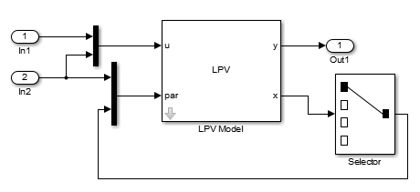
Consider a 2-input, 3-output, 4-state LPV model. Use input u(2) and state x(1) as scheduling parameters. Configure the Simulink^® model as shown in the following figure.

Simulate Linear Parameter-Varying System Using LPV System Block

Consider a linear mass-spring-damper system whose mass changes as a function of an external load command. The governing equation is as follows.

$$\mathit{m}\left(\mathit{u}\right)\ddot{\mathit{y}}+\mathit{c}\dot{\mathit{y}}+\mathit{ky}=\mathit{F}\left(\mathit{t}\right)$$

Here, $\mathit{m}\left(\mathit{u}\right)$ is the mass dependent upon the external command $\mathit{u}$, $\mathit{c}$ is the damping ratio, $\mathit{k}$ is the stiffness of the spring, and $\mathit{F}\left(\mathit{t}\right)$ is the forcing input. $\mathit{y}\left(\mathit{t}\right)$ is position of the mass at a given time $\mathit{t}$. For a fixed value of $\mathit{u}$, the system is linear and expressed as:

$$\mathit{A}=\left[\begin{array}{cc}0& 1\\ -\frac{\mathit{k}}{\mathit{m}}& -\frac{\mathit{c}}{\mathit{m}}\end{array}\right],$$

$$\mathit{B}=\left[\begin{array}{c}0\\ \frac{1}{\mathit{m}}\end{array}\right],$$

$$\mathit{C}=\left[\begin{array}{cc}1& 0\end{array}\right]$$

$$\begin{array}{l}\dot{\mathit{x}}=\mathit{Ax}+\mathit{Bu}\\ \mathit{y}=\mathit{Cx}\end{array}$$

where, $\mathit{x}=\left[\begin{array}{c}\mathit{y}\\ \dot{\mathit{y}}\end{array}\right]$ is the state vector and $\mathit{m}$ is the value of the mass for a given value of $\mathit{u}$.

In this example, you want to study the model behavior over a range of input values from 1 to 10 Volts. For each value of $\mathit{u}$, measure the mass and compute the linear representation of the system. Suppose, mass is related to the input by the relationship $\mathit{m}\left(\mathit{u}\right)=10\mathit{u}+0.1{\mathit{u}}^2$. For values of u ranging from 1 to 10 results in the following array of linear systems.

c = 5;   
k = 300; 
u = 1:10;
m = 10*u + 0.1*u.^2;
for i = 1:length(u)
   A = [0 1; -k/m(i), -c/m(i)];
   B = [0; 1/m(i)];
   C = [1 0];
   sys(:,:,i) = ss(A,B,C,0); 
end

The variable $\mathit{u}$ is the scheduling input. Add this information to the model.

sys.SamplingGrid = struct('LoadCommand',u);

Configure the LPV System block:

• Type sys in the State-space array field.

• Connect the input port par to a one-dimensional source signal that generates the values of the load command. If the source provides values between 1 and 10, the block uses interpolation to compute the linear model at a given time instance. Otherwise, the block uses extrapolation.

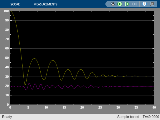
Simulate the LPV model to a constant forcing input of 100 N and random values for the load command scheduling variable.

model = "simMSDLPV";
open_system(model);

Compare Nonlinear Model and LPV Block Response

This example shows how to simulate a linear parameter-varying (LPV) model of an engine speed using the LPV System block. The LPV System block interpolates a state-space array to model the LPV response. Typically, you can obtain such an array by batch linearizing a nonlinear model over a range of operating conditions. This example provides a linearized result of the engine speed model in scdspeedlpvData. For more information about linearizing this model, see Linearize Engine Speed Model (Simulink Control Design).

Open the model.

model = "scdspeedLPVCompare";
open_system(model);

Load the linearization result for implementing the LPV model.

load scdspeedlpvData.mat

The LPV model is implemented under the LPV Model subsystem.

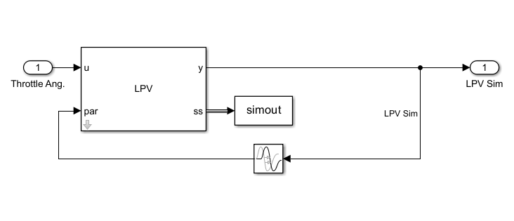
The LPV System block takes the throttle angle as an input and uses the speed output as scheduling variable. The block parameters are configured as shown in this image. Here, the state-space array sys and offsets are obtained by batch linearizing the nonlinear model.

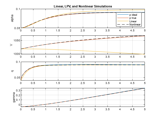
Simulate the model and plot the response comparison.

sim(model);
plot(logsOut{1}.Values.Time,logsOut{1}.Values.Data)
grid on
legend("Nonlinear sim","LPV sim","LTI sim",Location="best")

The LPV model provides a good approximation of the nonlinear response.

Extended Examples

LPV Approximation of Boost Converter Model

Approximate a nonlinear Simscape™ Electrical™ model using a linear parameter varying model.

Design and Validate Gain-Scheduled Controller for Nonlinear Aircraft Pitch Dynamics

Approximate nonlinear behavior of airframe pitch axis dynamics using linear parameter-varying model.

Open Live Script

Using LTI Arrays for Simulating Multi-Mode Dynamics

Construct a Linear Parameter Varying (LPV) representation of a system that exhibits multi-mode dynamics.

Open Script

Approximate Nonlinear Behavior Using Array of LTI Systems

You can use linear parameter varying models to approximate the dynamics of nonlinear systems.

Limitations

• Internal delays cannot be extrapolated to be less than their minimum value in the state-space model array.

• When using an scattered grid of linear models to define the LPV system, only the nearest neighbor interpolation scheme is used. This may reduce the accuracy of simulation results. It is recommended to work with rectangular grids created using ndgrid.

Ports

Input

u — Input signal

scalar | vector

Specify the input signal u(t). In multi-input case, this port accepts a signal of the dimension of the input.

par — Parameter values

scalar | vector

Provide the signals for variables defining the scheduling space (sampling grid variables). The scheduling variables can be functions of time, inputs and states, or constants. You can achieve the required dependence by preparing a scheduling signal using clock input (for time), input signal (u), the output state signals (x) of the LPV block, or any exogenous signals, as required.

Caution

Avoid making C(p) and D(p) depend on the system output y. Otherwise, the resulting state-space equation y = C(y)x + D(y)u creates an algebraic loop, because computing the output value y requires knowing the output value. This algebraic loop is prone to instability and divergence. Instead, try expressing C and D in terms of the time t, the block input u, and the state outputs x.

For similar reasons, avoid scheduling A(p) and B(p) based on the dx output. Note that it is safe to for A and B to depend on y when y is a fixed combination of states and inputs, (in other words, when y = Cx + Du where C and D are constant matrices).

Output

y — Model output

scalar | vector

Response of the linear parameter-varying model.

x — State values

scalar | vector

Values of the model states

Dependencies

To enable this port, select Output states on the Outputs tab of the block parameters.

dx — State derivative values

scalar | vector

Values of the state derivatives. The state derivatives are sometimes used to define the scheduling parameters. However, avoid scheduling A and B based on the dx output.

Dependencies

To enable this port, select Output state derivatives (continuous-time) or updates (discrete-time) on the Outputs tab of the block parameters.

ss — Local state-space model

bus

Local state-space model data at the major simulation time steps, returned as a bus signal with these elements.

• A — State matrix

• B — Input matrix

• C — Output matrix

• D — Feedthrough matrix

• InputDelay — Input delay

• OutputDelay — Output delay

• InternalDelay — Internal delays in the model

Dependencies

To enable this port, select Output interpolated state-space data on the Outputs tab of the block parameters.

offset — LPV model offsets

bus

LPV model offset data at the major simulation time steps, returned as a bus signal with these elements.

• InputOffset

• OutputOffset

• StateOffset

• StateDerivativeOffset

Dependencies

To enable this port, select Output interpolated offsets on the Outputs tab of the block parameters.

Parameters

To edit block parameters interactively, use the Property Inspector. From the Simulink Toolstrip, on the Simulation tab, in the Prepare gallery, select Property Inspector.

LPV Model Tab

State-space array — Array of state-space models

ss or idss model array

An array of state-space (ss or idss (System Identification Toolbox)) models. All the models in the array must use the same definition of states.

The state-space array must specify scheduling parameters and the interpolation grid for the model in the SamplingGrid property. You can also specify the model offsets in the Offsets property of the array when you set the Operating Point Offsets parameter to Use offsets in state-space array, See the ss model reference page for more information on these properties.

When the block is in a model with synchronous state control (see the State Control (HDL Coder) block), you must specify an array of discrete-time models.

Programmatic Use

To set the block parameter value programmatically, use the set_param (Simulink) function.

Parameter:	sys
Values:	ss or idss model array name in quotes

Example: set_param(gcb,"sys","sysArrayName")

Initial state — Initial conditions

0 (default) | vector

Initial conditions to use with the local model to start the simulation, specified as a vector of length equal to the number of model states.

Programmatic Use

To set the block parameter value programmatically, use the set_param (Simulink) function.

Parameter:	x0
Values:	"0" (default) | initial state values in quotes

Example: set_param(gcb,"x0","[0 0.1]")

Operating Point Offsets — Offset specification format

Specify Offsets as double arrays (default) | Specify offsets as struct array | Use offsets in state-space array

Since R2024a

Specify the format for operating point offsets.

• Specify Offsets as double arrays — Specify offsets using the Input offset, Output offset, State Offset, and State derivative/update offset parameters.

• Specify offsets as struct array — Specify offsets as a structure array with fields u, y, x, and dx specifying the input, output, state, and state derivative offsets, respectively.

• Use offsets in state-space array — Use the offsets specified in the Offsets property of the state-space array.

Programmatic Use

To set the block parameter value programmatically, use the set_param (Simulink) function.

Parameter:	opSpecOption
Values:	"Specify Offsets as double arrays" (default) | "Specify offsets as struct array" | "Use offsets in state-space array"

Example: set_param(gcb,"opSpecOption","Specify offsets as struct array")

Input offset — Input offset

0 (default) | array

Offsets in input u(t), specified as one of the following:

• 0 — Use when there are no input offsets ($\overline{u}\left(p\right)=0 \forall p$).

• Double vector of length equal to the number of inputs — Use when input offset is the same across the scheduling space.

• Double array of size n_u-by-1-by-N₁-by-...-by-N_m array — Use when offsets are present and they vary across the scheduling space. Here, n_u is the number of inputs and N₁-by-...-by-N_m is the size of the scheduling grid. For example, if your model has three inputs, two outputs, and four states and is scheduled over a 5-by-6 grid of operating points, the input array size must be 3-by-1-by-5-by-6. Use size(sys) to determine the size of the state-space array sys.

Dependencies

To enable this parameter, set the Operating Point Offsets format to Specify Offsets as double arrays.

Programmatic Use

To set the block parameter value programmatically, use the set_param (Simulink) function.

Parameter:	uOffset
Values:	"0" (default) | array name in quotes

Example: set_param(gcb,"uOffset","uOffArray")

Output offset — Output offset

0 (default) | array

Offsets in output y(t), specified as one of the following:

• 0 — Use when there are no output offsets $\overline{y}\left(p\right)=0 \forall p$.

• Double vector of length equal to the number of outputs. Use when output offsets are the same across the scheduling space.

• Double array of size n_y-by-1-by-N₁-by-...-by-N_m array — Use when offsets are present and they vary across the scheduling space. Here, n_y is the number of outputs and N₁-by-...-by-N_m is the size of the scheduling grid. For example, if your model has three inputs, two outputs, and four states and is scheduled over a 5-by-6 grid of operating points, the input array size must be 2-by-1-by-5-by-6. Use size(sys) to determine the size of the state-space array sys.

Dependencies

To enable this parameter, set the Operating Point Offsets format to Specify Offsets as double arrays.

Programmatic Use

To set the block parameter value programmatically, use the set_param (Simulink) function.

Parameter:	yOffset
Values:	"0" (default) | array name in quotes

Example: set_param(gcb,"yOffset","yOffArray")

State offset — State offset

0 (default) | array

Offsets in states x(t), specified as one of the following:

• 0 — Use when there are no state offsets $\overline{x}\left(p\right)=0 \forall p$.

• Double vector of length equal to the number of states. Use when the state offsets are the same across the scheduling space.

• Double array of size n_x-by-1-by-N₁-by-...-by-N_m array — Use when offsets are present and they vary across the scheduling space. Here, n_x is the number of states and N₁-by-...-by-N_m is the size of the scheduling grid. For example, if your model has three inputs, two outputs, and four states and is scheduled over a 5-by-6 grid of operating points, the input array size must be 4-by-1-by-5-by-6. Use size(sys) to determine the size of the state-space array sys.

Dependencies

To enable this parameter, set the Operating Point Offsets format to Specify Offsets as double arrays.

Programmatic Use

To set the block parameter value programmatically, use the set_param (Simulink) function.

Parameter:	xOffset
Values:	"0" (default) | array name in quotes

Example: set_param(gcb,"xOffset","xOffArray")

State derivative/update offset — State derivative or update offset

array

Offsets in state derivative or update variable dx(t), specified as one of the following:

• If you obtained the linear system array by linearization under equilibrium conditions, select the Assume equilibrium operating conditions option. This option corresponds to an offset of $\overline{dx}\left(p\right)=0$ for a continuous-time system and $\overline{dx}\left(p\right)=\overline{x}\left(p\right)$ for a discrete-time system. This option is selected by default.

• If the linear system contains at least one system that you obtained under non-equilibrium conditions, clear the Assume equilibrium operating conditions option. Specify one of the following in the Offset value field:

  • If the dx offset values are the same across the scheduling space, specify as a double vector of length equal to the number of states.

  • If the dx offsets are present and they vary across the scheduling space, specify as a double array of size n_x-by-1-by-N₁-by-...-by-N_m array — Use when offsets are present and they vary across the scheduling space. Here, n_x is the number of states and N₁-by-...-by-N_m is the size of the scheduling grid. For example, if your model has three inputs, two outputs, and four states and is scheduled over a 5-by-6 grid of operating points, the input array size must be 4-by-1-by-5-by-6. Use size(sys) to determine the size of the state-space array sys.

Dependencies

To enable this parameter, set the Operating Point Offsets format to Specify Offsets as double arrays and disable Assume equilibrium operating conditions.

Programmatic Use

To set the block parameter value programmatically, use the set_param (Simulink) function.

Parameter:	dxOffset
Values:	"0" (default) | array name in quotes

Example: set_param(gcb,"dxOffset","dxOffArray")

Struct array — Offsets structure array

struct (default) | structure array name

Since R2024a

Model offsets, specified as a structure with these fields.

Field	Description
u	Input offsets
y	Output offsets
x	State offsets
dx	State derivative offsets

• If offset values are the same across the scheduling space, specify as a double vector of length equal to the number of inputs, outputs, or states for the corresponding fields.

• If the offsets vary across scheduling space, specify a structure array. For instance, suppose that your model has three inputs, two outputs, and four states. If you linearize your model using a 5-by-6 array of operating points, the structure array size must be 5-by-6 and each entry must contain a vector of length equal to the number of inputs, outputs, or states for the corresponding fields.

The linearize (Simulink Control Design) function returns offsets in this format in the info.Offsets output when you linearize with StoreOffsets option set to true.

Dependencies

To enable this parameter, set the Operating Point Offsets format to Specify Offsets as struct array. (since R2024a)

Programmatic Use

To set the block parameter value programmatically, use the set_param (Simulink) function.

Parameter:	Offset
Values:	"struct" (default) | structure array name in quotes

Example: set_param(gcb,"Offset","OffsetStructName")

Fixed Entries Tab

Nominal model — Nominal LPV model

Use the first model in state-space array (default) | Custom value

State-space model that provides the values of the fixed coefficients, specified as one of the following:

• Use the first model in state-space array (Default:) — The first model in the state-space array is used to represent the LPV model. In the following example, the state-space array is specified by object sys and the fixed coefficients are taken from model sys(:,:,1).

  % Specify a 4-by-5 array of state-space models.
  sys = rss(4,2,3,4,5);
  a = 1:4; 
  b = 10:10:50;
  [av,bv] = ndgrid(a,b);
  % Use "alpha" and "beta" variables as scheduling parameters.
  sys.SamplingGrid = struct('alpha',av,'beta',bv);  

  Fixed coefficients are taken from the model sysFixed = sys(:,:,1), which corresponds to [alpha=1, beta=10]. If the (2,1) entry of A matrix is forced to be fixed, its value used during the simulation is sysFixed.A(2,1).

• Custom value — Specify a different state-space model for fixed entries. Specify a variable for the fixed model in the State space model field. The fixed model must use the same state basis as the state-space array in the LPV model.

Fixed Coefficient Indices — Fixed coefficients of state-space matrices

false or 0 (default) | true or 1 | logical matrix

Specify which coefficients of the state-space matrices and delay vectors are fixed.

Specify one of the following:

• Scalar Boolean (true or false), if all entries of a matrix are to be treated the same way.

  The default value is false for the state-space matrices and delay vectors, which means that they are treated as free.

• Logical matrix of a size compatible with the size of the corresponding matrix:

  State-space matrix	Size of fixed entry matrix
  A matrix	nx-by-nx
  B matrix	nx-by-nu
  C matrix	ny-by-nx
  D matrix	ny-by-nu
  Input delay	nu-by-1
  Output delay	ny-by-1
  Internal delay	ni-by-1

  where, n_u is the number of inputs, n_y is the number of outputs, n_x is the number of states, n_i is the length of internal delay vector.

• Numerical indices to specify the location of fixed entries. See sub2ind reference page for more information on how to generate numerical indices corresponding to a given subscript (i,j) for an element of a matrix.

Scheduling Tab

Interpolation method — Interpolation method

Linear (default) | Nearest | Flat

Interpolation method. Defines how the state-space data must be computed for scheduling parameter values that are located away from their grid locations.

Specify one of the following options:

• Flat — Choose the state-space data at the grid point closest, but not larger than, the current point. The current point is the value of the scheduling parameters at current time.

• Nearest — Choose the state-space data at the closest grid point in the scheduling space.

• Linear — Obtain state-space data by linear interpolation of the nearest 2d neighbors in the scheduling space, where d = number of scheduling parameters.

The default interpolation scheme is Linear for regular grids of scheduling parameter values. For irregular grids, the Nearest interpolation scheme is always used regardless of the choice you made. To learn more about regular and irregular grids, see Regular vs. Irregular Grids.

The Linear method provides the highest accuracy but takes longer to compute. The Flat and Nearest methods are good for models that have mode-switching dynamics.

Programmatic Use

To set the block parameter value programmatically, use the set_param (Simulink) function.

Parameter:	IMethod
Values:	"Linear" (default) | "Nearest" | "Flat"

Example: set_param(gcb,"IMethod","Flat")

Extrapolation method — Extrapolation method

Clip (default) | Linear

Extrapolation method. Defines how to compute the state-space data for scheduling parameter values that fall outside the range over which the state-space array has been provided (as specified in the SamplingGrid property).

Specify one of the following options:

• Clip (default) — Disables extrapolation and returns the data corresponding to the last available scheduling grid point that is closest to the current point.

• Linear — Fits a line between the first or last pair of values for each scheduling parameter, depending upon whether the current value is less than the first or greater than the last grid point value, respectively. This method returns the point on that line corresponding to the current value. Linear extrapolation requires that the interpolation scheme be linear too.

Programmatic Use

To set the block parameter value programmatically, use the set_param (Simulink) function.

Parameter:	EMethod
Values:	"Clip" (default) | "Linear"

Example: set_param(gcb,"EMethod","Linear")

Index search method — Prelookup algorithm

Binary search (default) | Linear search

The block determines the location of the current scheduling parameter values in the scheduling space using a prelookup algorithm. Select Linear search or Binary search. Each search method has speed advantages in different situations. For more information on this parameter, see the Prelookup (Simulink) block reference page.

Programmatic Use

To set the block parameter value programmatically, use the set_param (Simulink) function.

To get the block parameter value programmatically, use the get_param (Simulink) function.

Parameter:	IndexSearch
Values:	"Binary Search" (default) | "Linear Search"

Example: set_param(gcb,"IndexSearch","Linear Search")

Begin index search using previous index result — Begin search at previous time step

on (default) | off

Select this check box when you want the block to start its search using the index found at the previous time step. For more information on this parameter, see the Prelookup (Simulink) block reference page.

Programmatic Use

To set the block parameter value programmatically, use the set_param (Simulink) function.

Parameter:	IndexBegin
Values:	"on" (default) | "off"

Example: set_param(gcb,"IndexBegin","off")

Code Generation Tab

Block data type (discrete-time case only) — Block data type

double (default) | single

Block data type, specified as double or single.

Dependencies

To enable this option, use a discrete-time state-space model as input.

Programmatic Use

To set the block parameter value programmatically, use the set_param (Simulink) function.

Parameter:	DataType
Values:	"double" (default) | "single"

Example: set_param(gcb,"DataType","single")

Initial buffer size for delays — Initial buffer size

1024 (default) | positive integer greater than 5

Initial memory allocation for the number of input points to store for models that contain delays. If the number of input points exceeds the initial buffer size, the block allocates additional memory. The default size is 1024.

When you run the model in Accelerator mode or build the model, make sure the initial buffer size is large enough to handle maximum anticipated delay in the model.

Programmatic Use

To set the block parameter value programmatically, use the set_param (Simulink) function.

Parameter:	InitBufferSize
Values:	"1024" (default) | positive integer greater than 5 in quotes

Example: set_param(gcb,"InitBufferSize","512")

Use fixed buffer size — Use fixed buffer size

off (default) | on

Specify whether to use a fixed buffer size to save delayed input and output data from previous time steps. Use this option for continuous-time LPV systems that contain input or output delays. If the buffer is full, new data replaces data already in the buffer. The software uses linear extrapolation to estimate output values that are not in the buffer.

Programmatic Use

To set the block parameter value programmatically, use the set_param (Simulink) function.

Parameter:	FixedBuffer
Values:	"off" (default) | "on"

Example: set_param(gcb,"FixedBuffer","on")

Extended Capabilities

C/C++ Code Generation
Generate C and C++ code using Simulink® Coder™.

Version History

Introduced in R2014b

R2024a: Improved support for offsets and other enhancements

The LPV System block now supports specifying operating point offsets in two new formats:

• Specify offsets as struct array

• Use offsets in state-space array

Before R2024a, the block supported specifying offsets only as double arrays in the block parameters. Use the Operating Point Offsets list to specify the format of offsets.

Additionally, the block has the following new enhancements:

• The block architecture now uses a Varying State Space block underneath. This streamlines the support for offsets.

• The block now supports fast restart for simulation. In this mode, only the block inputs and the Initial state parameter are tunable. The rest of the block parameters are non tunable because changing them alters the model topology.

R2024a: Ignores constant parameters in SamplingGrid

The LPV System block now ignores singleton dimension and constant parameters in the sampling grid of the input model array. Therefore, you must not feed the parameters, that is, the fields of the SamplingGrid structure with constant values to the par port of the block. Use only the varying fields with this port.

Before R2024a, the block returned an error when fed parameters with constant values.