loopview

Graphically analyze MIMO feedback loops

Syntax

loopview(G,C) loopview(G,C,info)

Description

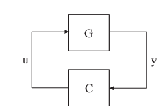
loopview(G,C) plots characteristics of the following positive-feedback, multi-input, multi-output (MIMO) feedback loop with plant G and controller C.

Use loopview to analyze the performance of a tuned control system you obtain using looptune.

Note

If you are tuning a Simulink^® model with looptune through an slTuner interface, analyze the performance of your control system using loopview (Simulink Control Design) for slTuner (requires Simulink Control Design™).

loopview plots the singular values of:

Open-loop frequency responses G*C and C*G
Sensitivity function S = inv(1-G*C) and complementary sensitivity T = 1-S
Maximum (target), actual (tuned), and normalized MIMO stability margins. loopview plots the multi-loop disk margin (see Stability Analysis Using Disk Margins (Robust Control Toolbox)). Use this plot to verify that the stability margins of the tuned system do not significantly exceed the target value.

For more information about singular values, see sigma.

loopview(G,C,info) uses the info structure returned by looptune. This syntax also plots the target and tuned values of tuning constraints imposed on the system. Additional plots include:

Singular values of the maximum allowed S and T. The curve marked S/T Max shows the maximum allowed S on the low-frequency side of the plot, and the maximum allowed T on the high-frequency side. These curves are the constraints that looptune imposes on S and T to enforce the target crossover range wc.
Target and tuned values of constraints imposed by any tuning goal requirements you used with looptune.

Use loopview with the info structure to assist in troubleshooting when tuning fails to meet all requirements.

Input Arguments

G

Numeric LTI model or tunable genss model representing the plant in a control system. The plant is the portion of a control system whose outputs are sensor signals (measurements), and whose inputs are actuator signals (controls).

You can obtain G as an output argument from looptune when you tune your control system.

C

genss model representing the controller in a control system. The controller is the portion of your control system that receives sensor signals (measurements) as inputs and produces actuator signals (controls) as outputs.

You can obtain C as an output argument from looptune when you tune your control system.

info

info structure returned by looptune during control system tuning.

Examples

collapse all

Examine Performance of Tuned Controller

Open Live Script

Tune a control system with looptune and use loopview to examine the performance of the tuned controller.

Create and tune control system.

s = tf('s');
G = 1/(75*s+1)*[87.8 -86.4; 108.2 -109.6];
G.InputName = {'qL','qV'};
G.OutputName = 'y';

D = tunableGain('Decoupler',eye(2));
PI_L = tunablePID('PI_L','pi');
PI_L.OutputName = 'qL';  
PI_V = tunablePID('PI_V','pi'); 
PI_V.OutputName = 'qV';

sum = sumblk('e = r - y',2);
C0 = (blkdiag(PI_L,PI_V)*D)*sum;

wc = [0.1,1];
options = looptuneOptions('RandomStart',5);
[G,C,gam,info] = looptune(-G,C0,wc,options);

Final: Peak gain = 0.956, Iterations = 28
Achieved target gain value TargetGain=1.

Examine the controller performance.

figure('Position',[100,100,520,1000])
loopview(G,C,info)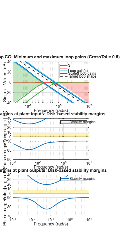

The first plot shows that the open-loop gain crossovers fall close to the specified interval [0.1,1]. This plot also includes the tuned values of the sensitivity function S = inv(1-G*C) and complementary sensitivity T = 1-S. These curves reflect the constraints that looptune imposes on S and T to enforce the target crossover range wc.

The second and third plots show that the MIMO stability margins of the tuned system fall well within the target range.

Alternatives

For analyzing Simulink models tuned with looptune through an slTuner (Simulink Control Design) interface, use loopview (Simulink Control Design) for slTuner (requires Simulink Control Design).