Visualize Antenna Field Strength Map on Earth
This example shows how to calculate an antenna's field strength on flat earth and display it on a map.
Create Helix
Use the default helix, and rotate it by 90 degrees so that most of its field is along the XY-plane, i.e. on the Earth's surface.
f0 = 2.4e9;
ant = helix(Tilt=-90);
f = figure;
show(ant)
view(-220,30)
title("Helix Antenna")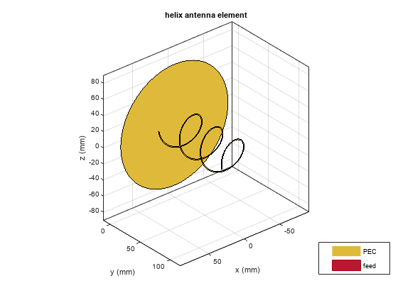
Calculate Electric Field at Various Points in Space
Assume the origin of the tilted antenna is located 15 m above the ground. Calculate the electric field in a rectangular region covering 500-by-500 km.
z = -15;
x = (-250:4:250)*1e3;
y = (-100:4:400)*1e3;

[X,Y] = meshgrid(x,y);
numpoints = length(x)*length(y);
points = [X(:)'; Y(:)'; z*ones(1,numel(X))];

E = EHfields(ant,f0,points); % Units: V/m
Calculate Magnitude of Electric Field
Compute the magnitude of the electric field.
Emag = zeros(1,numpoints);
for m=1:numpoints
    Emag(m) = norm(E(:,m)/sqrt(2));
end
Emag = 20*log10(reshape(Emag,length(y),length(x))); % Units: dBV/m
Emag = Emag + 120; % Units: dBuV/m
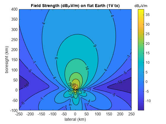
Plot Electric Field
Plot the magnitude of the electric field as a function of the x and y distance.
d_min = min(Emag(:));
d_max = max(Emag(:));
del = (d_max-d_min)/12;
d_vec = round(d_min:del:d_max);

if isvalid(f)
    close(f)
end
figure
contourf(X*1e-3,Y*1e-3,Emag,d_vec,showtext="on")
title("Field Strength (dB\muV/m) on flat Earth (1V tx)")
xlabel("lateral (km)")
ylabel("boresight (km)")
c = colorbar;
set(get(c,"title"),"string","dB\muV/m")
Define Transmitter Site with Antenna
Specify location and orientation of the antenna. Assign a location of 42 degrees north and 73 degrees west, along with antenna height of 15 meters. Orient the antenna toward the southwest at an angle of -150 degrees (or, equivalently, +210 degrees) measured counterclockwise from east.
lat =  42;
lon = -73;
h = 15;
az = -150;
Because the antenna points along the local Y-axis (not the X-axis), subtract 90 degrees to determine the rotation of the local system with respect to xEast-yNorth. (This is the angle to the local X-axis from xEast measured counterclockwise.)
xyrot = wrapTo180(az - 90);
Define a transmitter site with the antenna and orientation defined above.
tx = txsite(Name="Antenna Site",...
    Latitude=lat,...
    Longitude=lon,...
    Antenna=ant,...
    AntennaHeight=h,...
    AntennaAngle=xyrot,...
    TransmitterFrequency=f0);
Calculate Transmitter Power
Calculate root mean square value of power corresponding to antenna EH-fields calculation and set as transmitter power.
Z = impedance(tx.Antenna,tx.TransmitterFrequency);
If = feedCurrent(tx.Antenna,tx.TransmitterFrequency);
Irms = norm(If)/sqrt(2);
Ptx = real(Z)*(Irms)^2;
tx.TransmitterPower = Ptx;
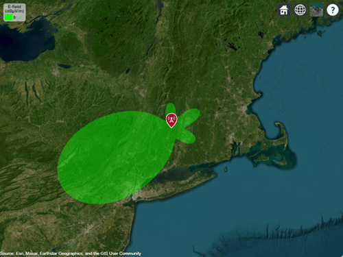
Display Electric Field Coverage Map with Single Contour
Show transmitter site marker on a map and display coverage zone. Specify a signal strength of 9 dBuV/m to display a single electric field contour. Specify the propagation model as 'freespace' to model idealized wave propagation in free space, which disregards obstacles due to curvature of the Earth or terrain.
% Launch Site Viewer with no terrain
viewer = siteviewer(Terrain="none");

% Plot coverage
coverage(tx,"freespace",...
    Type="efield",...
    SignalStrengths=9)
Customize Site Viewer
Set the map imagery using the Basemap property. Alternatively, open the map imagery picker in Site Viewer by clicking the second button from the right. Select "Topographic" to see topography and labels on the map.
viewer.Basemap = "topographic"; 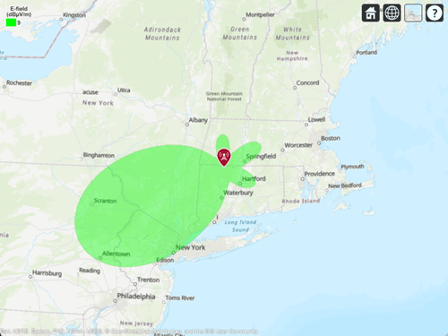
Display Electric Field Coverage Map with Multiple Contours
Specify multiple signal strengths to display multiple electric field contours.
sigStrengths = [9 14 19 24 29 36];
coverage(tx,"freespace",...
    Type="efield",...
    SignalStrengths=sigStrengths,...
    Colormap="parula",...
    ColorLimits=[9 36])

See Also
Functions
Objects
helix|siteviewer|txsite