Parallelization of Antenna and Array Analyses

Frequency Sweep Analysis

Analyzing antenna performance over a frequency band is an important part of antenna design. Port analyses include impedance, returnLoss, sparameters, vswr; surface analyses include current and charge; and field analyses include pattern, EHfields, axialRatio, and beamwidth. In this example, we demonstrate the advantages of parallel computing for computing axial ratio and return loss over a frequency band.

Axial Ratio Computation without Parallel Computing

Compute the axial ratio of an Archimedean spiral over a frequency band of 0.8 to 2.5 GHz in steps of 100 MHz. This calculation is done serially, and the time taken to perform these computations is saved in variable time1.

sp = spiralArchimedean(Turns=4,InnerRadius=5.5e-3,OuterRadius=50e-3);
freq = 0.8e9:100e6:2.5e9;
AR = zeros(size(freq));
tic
for m = 1:numel(freq)
    AR(m) = axialRatio(sp, freq(m), 0, 90);
end
time1 = toc;

Axial Ratio Computation with Parallel Computing

Repeat the calculations using Parallel Computing Toolbox to reduce computation time. Use the function parpool to create a parallel pool cluster. Then, use parfor to calculate the axial ratio over the same frequency band. The time taken to perform the computation is saved in variable time2.

pardata = parpool;

Starting parallel pool (parpool) using the 'Processes' profile ...
Connected to parallel pool with 8 workers.

sp = spiralArchimedean(Turns=4,InnerRadius=5.5e-3,OuterRadius=50e-3);
ARparfor = zeros(size(freq));
tic;
parfor m = 1:numel(freq)
    ARparfor(m) = axialRatio(sp, freq(m), 0, 90);
end
time2 = toc;

Axial Ratio Computation Time Comparison

The table below shows the time taken for axial ratio analysis with and without Parallel Computing Toolbox. The cluster information is saved in the variable pardata.

cases = {'Without Parallel Computing';'With Parallel Computing'};
time  = [time1; time2];
numWorkers = [1; pardata.NumWorkers];
disp(table(time,numWorkers,RowNames=cases))

                                   time     numWorkers
                                  ______    __________

    Without Parallel Computing    7.8362        1     
    With Parallel Computing       7.0631        8     

fprintf('Speed-up due to parallel computing = %g', time1/time2)

Speed-up due to parallel computing = 1.10945

The plot below shows the axial ratio data calculated for two cases. The results are identical.

plot(freq./1e9, AR,'r+', freq./1e9, ARparfor,'bo');
grid on;
xlabel("Frequency (GHz)");
ylabel("Axial ratio (dB)");
title("Axial ratio of Archimedean spiral antenna at boresight");
legend("Without Parallel Computing","With Parallel Computing", ...
    location="Best");

During this analysis the antenna structure is meshed at every frequency and then the far-fields are computed at that frequency to compute the axial ratio. One way of reducing the analysis time is to mesh the structure manually by specifying a maximum edge length.

Return Loss Computation without Parallel Computing

The previous section performed a field analysis computation. All field and surface analysis computations in Antenna Toolbox™ accept only scalar frequency as input. Whereas, returnLoss and all other port analysis functions accept a frequency vector as input.

When a frequency vector is specified as an input, the antenna structure is meshed at the highest frequency. The resulting mesh is used for performing the analysis over the specified frequency band. The CPU time taken to perform the computation is saved in variable time3.

sp = spiralArchimedean(Turns=4,InnerRadius=5.5e-3,OuterRadius=50e-3);
tic;
RL = returnLoss(sp, freq);
time3 = toc;

Return Loss Computation with Parallel Computing

If we use the parfor loop by passing a single frequency at a time (as shown in the discussion about axialRatio), the meshing will happen at every frequency. This will limit the advantage of parallel computing. A better option is to manually mesh the structure and then use the parfor loop to run a frequency sweep. A simple way to do this is to run the analysis at the highest frequency first and get the mesh information using the mesh function. Use the maximum edge length in the mesh function to ensure that the same mesh is used for all computations. The time taken to perform the computation is saved in variable time4.

sp = spiralArchimedean(Turns=4,InnerRadius=5.5e-3,OuterRadius=50e-3);
RLparfor = zeros(size(freq));
tic;
temp = returnLoss(sp, freq(end));
meshdata = mesh(sp);
[~] = mesh(sp, MaxEdgeLength=meshdata.MaxEdgeLength);
parfor m = 1:numel(freq)
    RLparfor(m) = returnLoss(sp, freq(m)); 
end
time4 = toc;

Return Loss Computation Time Comparison

The table below indicated the time taken for calculating the return loss with and without Parallel Computing Toolbox. The cluster information is saved in the variable pardata.

cases = {'Without Parallel Computing';'With Parallel Computing'};
time  = [time3; time4];
numWorkers = [1; pardata.NumWorkers];
disp(table(time,numWorkers,RowNames=cases))

                                   time      numWorkers
                                  _______    __________

    Without Parallel Computing     1.7048        1     
    With Parallel Computing       0.79786        8     

fprintf('Speed-up due to parallel computing = %g', time3/time4);

Speed-up due to parallel computing = 2.13665

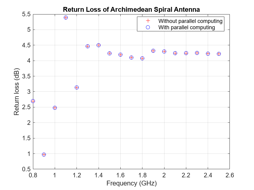
The plot below shows the return loss data calculated for two cases. The results are identical.

plot(freq./1e9, RL,'r+', freq./1e9, RLparfor,'bo');
grid on;
xlabel("Frequency (GHz)");
ylabel("Return loss (dB)");
title("Return loss of Archimedean spiral antenna");
legend("Without Parallel Computing","With Parallel Computing", ...
     location="Best");

Delete the current parallel pool.

delete(gcp);