Modeling Resonant Coupled Wireless Power Transfer System
This example shows how to create and analyze a resonant coupling type wireless power transfer (WPT) system with an emphasis on concepts such as resonant mode, coupling effect, and magnetic field pattern. The analysis is based on a two-element system of spiral resonators.
Design Frequency and System Parameters
Choose the design frequency to be 30 MHz. This is a popular frequency for compact WPT system design. Also specify the frequency for broadband analysis, and the points in space to plot near fields.
fc = 30e6;
fcmin = 28e6;
fcmax = 31e6;
fband1 = 27e6:1e6:fcmin;
fband2 = fcmin:0.25e6:fcmax;
fband3 = fcmax:1e6:32e6;
freq = unique([fband1 fband2 fband3]);
pt=linspace(-0.3,0.3,61);
[X,Y,Z]=meshgrid(pt,0,pt);
field_p=[X(:)';Y(:)';Z(:)'];
The Spiral Resonator
The spiral is a very popular geometry in a resonant coupling type wireless power transfer system for its compact size and highly confined magnetic field. We will use such a spiral as the fundamental element in this example.
Create Spiral Geometry
The spiral is defined by its inner and outer radius, and number of turns.
Rin = 0.05;
Rout = 0.15;
N = 6.25;
spiralobj = spiralArchimedean(NumArms=1,Turns=N,...
    InnerRadius=Rin,OuterRadius=Rout,Tilt=90,TiltAxis="Y");
Resonance Frequency and Mode
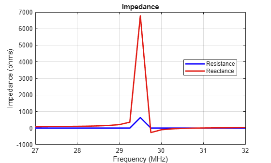
It is important to find the resonant frequency of the designed spiral geometry. A good way to find the resonant frequency is to study the impedance of the spiral resonator. Since the spiral is a magnetic resonator, a lorentz shaped reactance is expected and observed in the calculated impedance result.
figure
impedance(spiralobj,freq);
Since the spiral is a magnetic resonator, the dominant field component of this resonance is the magnetic field. A strongly localized magnetic field is observed when the near field is plotted.
figure
EHfields(spiralobj,fc,field_p,ViewField='H',ScaleFields=[0 5]);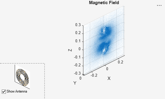
Create Spiral to Spiral Power Transfer System
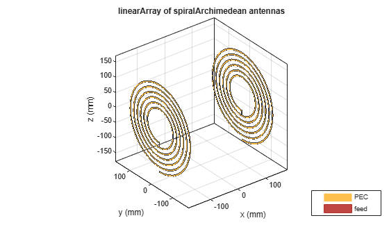
The complete wireless power transfer system is composed of two parts: the transmitter(Tx) and receiver(Rx). Choose identical resonators for both transmitter and receiver to maximize the transfer efficiency. Here, the wireless power transfer system is modeled as a linear array.
wptsys = linearArray(Element=[spiralobj spiralobj]);
wptsys.ElementSpacing = Rout*2;
figure
show(wptsys)
Variation of System Efficiency with Transfer Distance
One way to evaluate the efficiency of the system is by studying the S21 parameter. As presented in [[1]], the system efficiency changes rapidly with operating frequency and the coupling strength between the transmitter and receiver resonator. Peak efficiency occurs when the system is operating at its resonant frequency, and the two resonators are strongly coupled.
sparam = sparameters(wptsys,freq);
figure
rfplot(sparam,2,1,"abs");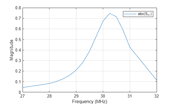
Critical Coupled Point
The coupling between two spirals increases with decreasing distance between two resonators. This trend is approximately proportional to . Therefore, the system efficiency increases with shorter transfer distance until it reaches the critical coupled regime [1]. When the two spirals are over coupled, exceeding the critical coupled threshold, system efficiency remains at its peak, as shown in Fig.3 in [1]. We observe this critical coupling point and over coupling effect during modeling of the system. Perform a parametric study of the system s-parameters as a function of the transfer distance. The transfer distance is varied by changing the ElementSpacing. It is varied from half of the spiral dimension to one and half times of the spiral dimension, which is twice of the spiral's outer radius. The frequency range is expanded and set from 25 MHz to 36 MHz.
freq = (25:0.1:36)*1e6;
dist = Rout*2*(0.5:0.1:1.5);

load("wptData.mat");
s21_dist = zeros(length(dist),length(freq));
for i = 1:length(dist)
    s21_dist(i,:) = rfparam(sparam_dist(i),2,1);
end

figure;
[X,Y] = meshgrid(freq/1e6,dist);
surf(X,Y,abs(s21_dist),EdgeColor="none");
view(150,20);
shading(gca,"interp");
axis tight;
xlabel("Frequency [MHz]");
ylabel("Distance [m]");
zlabel("S_{21} Magnitude");
![Figure contains an axes object. The axes object with xlabel Frequency [MHz], ylabel Distance [m] contains an object of type surface.](../../examples/antenna/win64/atx_wireless_power_transfer_05.png)
Coupling Mode between Two Spiral Resonator
The dominant energy exchange mechanism between the two spiral resonators is through the magnetic field. Strong magnetic fields are present between the two spirals at the resonant frequency.
wptsys.ElementSpacing = Rout*2;
figure
EHfields(wptsys,fc,field_p,ViewField='H',ScaleFields=[0 5]);
view(0,0);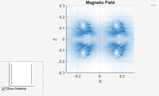
Animate the H-field Coupling
The analysis from the solver provides us with the steady state result. The field calculation provides the 3 components of the magnetic field in phasor form in cartesian coordinate system. Animate this field by using a propagator defined by the frequency, fc to bring the result back to time-harmonic form and visualize on the same slice plane XZ either of the components Hx or Hz. To do so use the helperAnimateEHFields function as shown below. Define the spatial extent, point density as well as the total number of time periods defined in terms of the frequency fc. If the sampling time is not defined, the function automatically chooses a sampling time based on 10 times the center frequency. There is also an option available to save the animation output to a gif file with an appropriate name specified.
% Excite the first resonator only
wptsys.AmplitudeTaper = [1 0];
% Define Spatial Plane Extent
SpatialInfo.XSpan = 2;
SpatialInfo.YSpan = 2;
SpatialInfo.ZSpan = 2;
SpatialInfo.NumPointsX = 200;
SpatialInfo.NumPointsY = 200;
SpatialInfo.NumPointsZ = 200;
% Define Time Extent
Tperiod = 1/fc;
T = 2*Tperiod;
TimeInfo.TotalTime = T;
TimeInfo.SamplingTime = [];             % Leave it empty for picking automatically
% Define Field Data details
DataInfo.Component = 'Hx';
DataInfo.PlotPlane = 'XZ';
DataInfo.DataLimits = [-0.25 0.5];
DataInfo.ScaleFactor = 1;
DataInfo.GifFileName = 'wptcpl.gif';
DataInfo.CloseFigure = true;
%% Animate
helperAnimateEHFields(wptsys,fc,SpatialInfo, TimeInfo, DataInfo)
Conclusion
The results obtained for the wireless power transfer system match well with the results published in [[1]].
References
[1] Sample, Alanson P, D A Meyer, and J R Smith. “Analysis, Experimental Results, and Range Adaptation of Magnetically Coupled Resonators for Wireless Power Transfer.” IEEE Transactions on Industrial Electronics 58, no. 2 (February 2011): 544–54. https://doi.org/10.1109/TIE.2010.2046002.