EVM Measurement of 5G NR PUSCH Waveforms
This example shows how to measure the error vector magnitude (EVM) of PUSCH fixed reference channel (FRC) waveforms. The example also shows how to add RF impairments, including in-phase and quadrature (I/Q) imbalance, phase noise and memoryless nonlinearity.
Introduction
For base station receiver RF testing, the 3GPP 5G NR standard defines a set of FRC waveforms. The FRCs for frequency range 1 (FR1) and frequency range 2 (FR2) are defined in TS 38.104, Annex A.
This example shows how to generate an NR waveform (FRC) and add impairments. The example uses in-phase and quadrature (I/Q) imbalance, phase noise and memoryless nonlinearities. It shows how to calculate the EVM of the resulting signal, and then plot the root mean square (RMS) and peak EVMs per orthogonal frequency division multiplexing (OFDM) symbol, slot, and subcarrier. Then calculate the overall EVM (RMS EVM averaged over the complete waveform). Annex F of TS 38.101-1 and TS 38.101-2 define an alternative method for computing the EVM in FR1 and FR2, respectively. The figure below shows the processing chain implemented in this example.
Simulation Parameters
Select one of the FRCs for FR1 and FR2.
rc ="G-FR1-A1-7"; % FRC % Possible overrides to Annex A definitions (empty values provide the Annex A defaults) bw = []; % Bandwidth override (5,10,15,20,25,30,40,50,60,70,80,90,100,200,400,800,1600,2000 MHz) scs = []; % Subcarrier spacing override (15,30,60,120,480,960 kHz) dm = []; % Duplexing mode override ("FDD","TDD") ncellid = []; % Cell identity override (used to control scrambling identities)
To print EVM statistics, set displayEVM to true. To disable the prints, set displayEVM to false. To plot EVM statistics, set plotEVM to true. To disable the plots, set plotEVM to false.
displayEVM =true; plotEVM =
true; if displayEVM fprintf('Reference Channel = %s\n',rc); end
Reference Channel = G-FR1-A1-7
To measure EVM as defined in TS 38.101-1 (FR1) or TS 38.101-2 (FR2), Annex F respectively, set evm3GPP to true. evm3GPP is disabled by default.
evm3GPP =  false;
To generate the waveform, create a waveform generator object. To change the configuration parameters, make them writable using the makeConfigWritable function.
wavegen = hNRReferenceWaveformGenerator(rc,bw,scs,dm,ncellid);
[txWaveform,tmwaveinfo,resourcesinfo] = generateWaveform(wavegen,wavegen.Config.NumSubframes);
Impairment: In-Phase and Quadrature (I/Q) Imbalance, Phase Noise and Memoryless Nonlinearity
This example considers the most typical impairments that distort the waveform when passing through an RF transmitter or receiver: phase noise, I/Q imbalance, and memoryless nonlinearity. Enable or disable impairments by toggling the flags phaseNoiseOn, IQImbalanceON, and nonLinearityModelOn.
phaseNoiseOn =true; IQImbalanceON =
true; nonLinearityModelOn =
true;
Normalize the waveform to fit the dynamic range of the nonlinearity.
txWaveform = txWaveform/max(abs(txWaveform),[],'all');The waveform consists of one frame for frequency division duplexing (FDD) and two for time division duplexing (TDD). Repeat the signal twice. For this example, remove the first half of the resulting waveform to avoid the transient introduced by the phase noise model.
txWaveform = repmat(txWaveform,2,1);
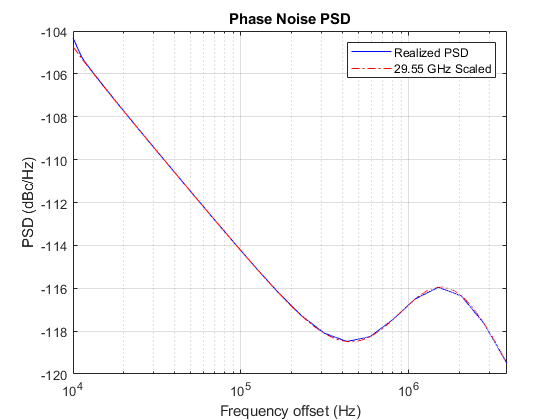
Introduce phase noise distortion. The figure shows the phase noise characteristic. The carrier frequency considered depends on the frequency range. We use values of 4 GHz and 28 GHz for FR1 and FR2, respectively. The phase noise characteristic is generated with the multipole zero model described in TR 38.803 Section 6.1.10.
if phaseNoiseOn
    sr = tmwaveinfo.Info.SamplingRate;

    % Carrier frequency
    if wavegen.Config.FrequencyRange == "FR1" % Carrier frequency for FR1
        fc = 4e9;
    else % Carrier frequency for FR2
        fc = 28e9;
    end

    % Apply phase noise to the waveform and visualize phase noise PSD
    pnoise = hNRPhaseNoise(fc,sr,MinFrequencyOffset=1e4,...
        RandomStream="mt19937ar with seed");
    visualize(pnoise);
    rxWaveform = zeros(size(txWaveform),'like',txWaveform);
    for i = 1:size(txWaveform,2)
        rxWaveform(:,i) = pnoise(txWaveform(:,i));
        release(pnoise)
    end
else
    rxWaveform = txWaveform; %#ok<UNRCH>
end
Introduce I/Q imbalance. Apply a 0.2 dB amplitude imbalance and a 0.5 degree phase imbalance to the waveform. You can also increase the amplitude and phase imbalances by setting amplitudeImbalance and phaseImbalance to higher values.
if IQImbalanceON
    amplitudeImbalance = 0.2;
    phaseImbalance = 0.5;
    rxWaveform = iqimbal(rxWaveform,amplitudeImbalance,phaseImbalance);
end
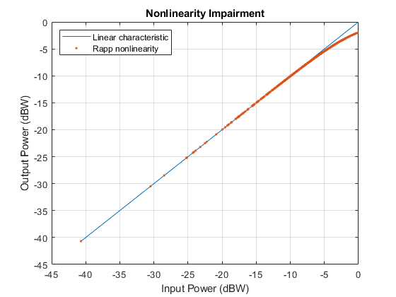
Introduce nonlinear distortion. For this example, use the Rapp model. The figure shows the introduced nonlinearity. Set the parameters for the Rapp model to match the characteristics of the memoryless model from TR 38.803 "Memoryless polynomial model - Annex A.1".
if nonLinearityModelOn
    rapp = comm.MemorylessNonlinearity('Method','Rapp model');
    rapp.Smoothness = 1.55;
    rapp.OutputSaturationLevel = 1;

    % Plot nonlinear characteristic
     plotNonLinearCharacteristic(rapp);

    % Apply nonlinearity
    for i = 1:size(rxWaveform,2)
        rxWaveform(:,i) = rapp(rxWaveform(:,i));
        release(rapp)
    end
end

The signal was previously repeated twice. Remove the first half of this signal to avoid any transient introduced by the impairment models.
dm = wavegen.ConfiguredModel{4};
if dm == "FDD"
    nFrames = 1;
else % TDD
    nFrames = 2;
end
rxWaveform(1:nFrames*tmwaveinfo.Info.SamplesPerSubframe*10,:) = [];
Measurements
The function, hNRPUSCHEVM, performs these steps to decode and analyze the waveform:
Coarse frequency offset estimation and correction
Integer frequency offset estimation and correction
I/Q imbalance estimation and correction
Synchronization using the demodulation reference signal (DM-RS) over one frame for FDD (two frames for TDD)
Direct current (DC) offset estimation and correction
OFDM demodulation of the received waveform
Fine frequency offset estimation and correction
DC subcarrier exclusion
Channel estimation
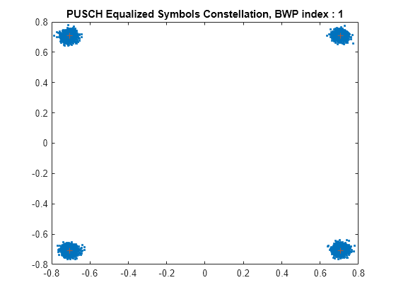
Equalization
Common phase error (CPE) estimation and compensation
PUSCH EVM computation (enable the switch
evm3GPPto process according to the EVM measurement requirements specified in TS 38.101-1(FR1) or TS 38.101-2 (FR2), Annex F.PUSCH power per resource element (RE)
PUSCH DM-RS EVM computation
PUSCH DM-RS power per RE
PUSCH PT-RS EVM computation
PUSCH PT-RS power per RE
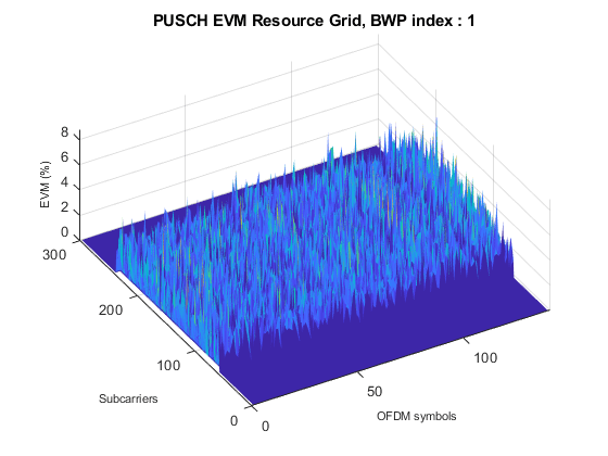
The example measures and outputs various EVM related statistics per symbol, per slot, and per frame peak EVM and RMS EVM. The example displays the EVM for each slot and frame, and displays the overall EVM averaged over the entire input waveform. The example produces these plots: EVM versus per OFDM symbol, slot, subcarrier, overall EVM and in-band emissions. Each EVM related plot displays the peak versus RMS EVM.
% Compute and display EVM measurements
cfg = struct();
cfg.Evm3GPP = evm3GPP;
cfg.PlotEVM = plotEVM;
cfg.DisplayEVM = displayEVM;
cfg.IQImbalance = IQImbalanceON;
[evmInfo,eqSym,refSym] = hNRPUSCHEVM(wavegen.Config,rxWaveform,cfg);
EVM stats for BWP idx : 1 RMS EVM, Peak EVM, slot 0: 2.285 8.015% DM-RS RMS EVM, Peak EVM, slot 0: 1.143 2.898% RMS EVM, Peak EVM, slot 1: 2.060 5.594% DM-RS RMS EVM, Peak EVM, slot 1: 1.584 4.318% RMS EVM, Peak EVM, slot 2: 2.095 5.766% DM-RS RMS EVM, Peak EVM, slot 2: 1.395 3.697% RMS EVM, Peak EVM, slot 3: 2.108 6.269% DM-RS RMS EVM, Peak EVM, slot 3: 1.363 3.200% RMS EVM, Peak EVM, slot 4: 2.180 5.978% DM-RS RMS EVM, Peak EVM, slot 4: 1.837 5.838% RMS EVM, Peak EVM, slot 5: 2.031 5.469% DM-RS RMS EVM, Peak EVM, slot 5: 1.154 2.526% RMS EVM, Peak EVM, slot 6: 2.230 7.946% DM-RS RMS EVM, Peak EVM, slot 6: 1.945 5.022% RMS EVM, Peak EVM, slot 7: 2.194 7.539% DM-RS RMS EVM, Peak EVM, slot 7: 1.627 3.981% RMS EVM, Peak EVM, slot 8: 2.083 6.691% DM-RS RMS EVM, Peak EVM, slot 8: 1.375 2.817% RMS EVM, Peak EVM, slot 9: 2.556 7.942% DM-RS RMS EVM, Peak EVM, slot 9: 1.422 3.515% Averaged RMS EVM frame 0: 2.187% Averaged overall RMS EVM: 2.187%


Peak EVM : 8.0145%
References
[1] TR 38.803 V14.3.0. "Study on new radio access technology: Radio Frequency (RF) and co-existence aspects." 3rd Generation Partnership Project; Technical Specification Group Radio Access Network.
[2] TS 38.104. "NR; Base Station (BS) radio transmission and reception." 3rd Generation Partnership Project; Technical Specification Group Radio Access Network.
[3] TS 38.101-1. "NR; User Equipment (UE) radio transmission and reception; Part 1: Range 1 Standalone." 3rd Generation Partnership Project; Technical Specification Group Radio Access Network.
[4] TS 38.101-2. "NR; User Equipment (UE) radio transmission and reception; Part 2: Range 2 Standalone." 3rd Generation Partnership Project; Technical Specification Group Radio Access Network.
Local Functions
function plotNonLinearCharacteristic(memoryLessNonlinearity)
    % Plot the nonlinear characteristic of the power amplifier (PA) impairment
    % represented by the input parameter memoryLessNonlinearity, which is a
    % comm.MemorylessNonlinearity Communications Toolbox(TM) System object.

    % Input samples
    x = complex((1/sqrt(2))*(-1+2*rand(1000,1)),(1/sqrt(2))*(-1+2*rand(1000,1)));

    % Nonlinearity
    yRapp = memoryLessNonlinearity(x);
    % Release object to feed it a different number of samples
    release(memoryLessNonlinearity);

    % Plot characteristic
    figure;
    plot(10*log10(abs(x).^2),10*log10(abs(x).^2));
    hold on;
    grid on
    plot(10*log10(abs(x).^2),10*log10(abs(yRapp).^2),'.');
    xlabel('Input Power (dBW)');
    ylabel('Output Power (dBW)');
    title('Nonlinearity Impairment')
    legend('Linear characteristic', 'Rapp nonlinearity','Location','Northwest');
end