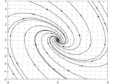
Phase Portrait Plotter on 2D phase plane
Version 1.0.3 (370 KB) by
Yu Zhang
This function could plot the phase portrait of the 2-dimentional autonomous system, and is configurable for arrows, vector fileds, etc.
Usage
Please open plotpp_example.mlx which contains three examples. If you do not have a live editor with your matlab version, then the following content might be useful to you.
In the first example, we only need one single command to get the phase portrait.
plotpp(@(t,x)[x(2);-x(1)-1*x(2)])

In the second example, we plot the phase portrait of the van der Pol equation:
We set the time span to 20 second, which is a proper time for demonstration, by trail and error. And we changed the color of quiver and lines to have a nice look.
odefun = @(t, x) [x(2); -x(1) + 0.5*(1 - x(1)^2)*x(2)];
plotpp(odefun,'tspan', 30,...
'quivercolor', [0.6,0.6,0.6],...
'linecolor', [0.3,0.3,0.3])

The third example is the swing equation:
We only want to plot the trajectories from the saddle to know where the region of attraction (ROA) is. Therefore, we set the input argument 'plotNonSaddleTrajectory' be false. We also set the solver region be  for δ and
  for ω, and set the minimum arrow density on trajectory, as are indicated by the arguments. Besides, to plot the trajectory of the unstable manifold of the left UEP, which converges to the left SEP, we set the axisMarginRatio to 0.5(scaled) so that the integration wouldn't stop on it, and hence we could get a complete trajectory towards the left SEP. Moreover, we do not want to display the quiver of the vector field, so we switch 'plotQuiver' off.
odefun = @(t, x) [x(2); 0.5 - sin(x(1)) - 0.2*x(2)];
plotpp(odefun, 'plotNonSaddleTrajectory', false, 'arrowSize', 12,...
'plotQuiver', false, 'axisMarginRatio', 0.5,...
'arrowDensity', 0.1,...
'xlim', [-2*pi, 2*pi], 'ylim', [-3, 3])
To generate a nice-look figure for publishing paper, we add more commands to decorate the figure, e.g., resizing the figure, and using Latex commands.
set(gcf, 'unit', 'centimeters', 'position', [0,0,14,8])
set(gca, 'ticklabelinterpreter', 'latex',...
'xtick', -2*pi:pi:2*pi,...
'xticklabels', {'$$-2\pi$$','$$-\pi$$',...
'$$0$$','$$\pi$$','$$\delta\mathrm{(rad)}$$'});
ylabel('$$\omega\mathrm{(p.u.)}$$', 'interpreter', 'latex');
legend({'Trajectory'}, 'Interpreter',"latex", 'location', 'northwest')

More Information
If you have any questions about plotpp, please refer to the help doc, which contains the detailed definition of the input arguments:
help plotpp
Then the following information will be displayed, which would be helpful for configuration. More configurable options might be deployed in the future.
Parameter definitions:
-- odefun: (required) this function must be a 2-dimension autonomous
function with respect to (t, x).
-- tspan: time span for ode computing, default value is 40;
-- xLim: x-axis plot range, default value is [-5,5];
-- yLim: y-axis plot range, default value is [-5,5];
-- xPlotNum: trajectories that start/end from horizental border,
default value is 4;
-- yPlotNum: trajectories that start/end from vertical border,
default value is 4;
-- lineColor: color of lines and points, default is [0.1,0.1,0.1];
-- quiverColor: color of quiver plots, default is [0.5,0.5,0.5]
-- plotNonSaddleTrajectory: whether or not to plot non-saddle points
trajcetories, default value is true;
-- plotEPs: whether or not to plot equilibrium points (EPs),
default value is true;
-- plotArrows: whether or not to plot arrows, default value is true;
-- plotQuiver: whether or not to plot quiver, default value is true.
-- arrowDensity: density arrows on each trajectory, default is 2,
and the minimum should be 0.1;
-- arrowSize: Size of arrows on the trajectory, default is 9;
-- axisMarginRatio: axis margin for solver so that the solver would not
stop when the trajectory crosses the axis limitation
until it crosses the axis margin border, which is
outside the axis limitation, default is 0.1;
Acknowledgement
The author is grateful to the author who contribute to the matlab function phasePortraitPlot.m, which enlighted me on how to add arrows on the phase portrait. I used some code pieces of yours, but I couldn't find tags in Matlab file exchanges. The author would also like to thank the author of package arrow and Phase Portrait Plotter for reliance and enlightening.
Cite As
Yu Zhang (2024). Phase Portrait Plotter on 2D phase plane (https://www.mathworks.com/matlabcentral/fileexchange/110785-phase-portrait-plotter-on-2d-phase-plane), MATLAB Central File Exchange. Retrieved .
MATLAB Release Compatibility
Created with
R2019a
Compatible with any release
Platform Compatibility
Windows macOS LinuxTags
Acknowledgements
Inspired by: arrow, Phase Portrait Plotter
Community Treasure Hunt
Find the treasures in MATLAB Central and discover how the community can help you!
Start Hunting!Discover Live Editor
Create scripts with code, output, and formatted text in a single executable document.

