I want to represent the temperature variation at specific points of the equatorial atlantic ocean

I would like to make a card like the one in the picture
clear all; close all; clc
ncfile = ('example.nc'); %loads temperature file
ncdisp(ncfile) %info about ncfile
sst = ncread(ncfile, 'to');
lon = ncread(ncfile,'longitude');
lat = ncread(ncfile,'latitude');
% Read in the sea_ice_fraction data and store in a new variable called ice:
%gets sea surface temperature value
time = ncread(ncfile,'time') ; nt = length(time) ; %reads the time variable and obtains its size
[X,Y] = meshgrid(lon,lat) ; % transform longitudes and latitudes into a grid of lon long x lat dimension
%%generates map
figure('Color','white'); %creates figure
ax=worldmap([55 70],[50 52]); % loads world map with the limits for atlantic ocean
newx= reshape(X, 383, 523);
nsst = permute(data,[1 3 2]);
nsst = reshape(nsst,[],size(data,2),1);
nsst= reshape(data, []);
%setm(ax,'mapprojection','mercator','Origin', [180 0 180]) %changes projection and changes origin reference for coordinates
levels=[ 1 2 3 4 5 6 7 8 9 10 11 12 13 14 15 16 17 18 19 20 21 22 ]; % creates levels for contours
geoshow(double(Y),double(X),nsst,'DisplayType','texturemap') %creates surface map of temperature
cb = contourcbar('peer',ax,'Location','northoutside'); %creates colorbar
caxis([15 35]) %defines limits for colorbar
colormap(jet) %sets color scheme
set(get(cb,'XLabel'),'String','SST (^oC)') %title for color bar
set(cb,'Position',[0.23 0.2417 0.5750 0.0335]) %adjust location and size of color bar
%levels=[28]; %sets level for contour defining specific
geoshow(double(Y),double(X),data,'DisplayType', 'contour','LevelList',levels,'LineColor','black') %plots temperature contour defining the western Pacific Warm Pool
hold on
land = shaperead('landareas.shp', 'UseGeoCoords', true); %define land areas
geoshow(land, 'FaceColor', [0 0 0]) % plots land areas in black

 Accepted Answer
unzip example.zip
ncfile = ('example.nc'); %loads temperature file
ncdisp(ncfile) %info about ncfile
Source: /users/mss.system.thlvCp/example.nc Format: classic Global Attributes: description = 'ARMOR3D NRT CMEMS December 2020 Release' title = 'ARMOR3D NRT - TSHUVMld Global Ocean Observation-based Product' Conventions = 'CF-1.0' institution = 'CLS' domain_name = 'GLO' history = '2023-08-02 00:00:00 ARMOR3D NRT - TSHUV Global Ocean Observation-based Product netCDF creation' _CoordSysBuilder = 'ucar.nc2.dataset.conv.CF1Convention' references = ' ' comment = '' source = ' ' Dimensions: time = 53 latitude = 31 longitude = 26 depth = 1 Variables: mlotst Size: 26x31x53 Dimensions: longitude,latitude,time Datatype: int16 Attributes: _FillValue = 32767 scale_factor = 0.1 unit_long = 'meter' add_offset = 2500 long_name = 'Mixed layer depth from min of temperature and density threshold equivalent to a 0.2C decrease' standard_name = 'ocean_mixed_layer_thickness' units = 'm' _ChunkSizes = [1 689 1440] depth Size: 1x1 Dimensions: depth Datatype: int16 Attributes: axis = 'Z' long_name = 'depth' positive = 'down' standard_name = 'depth' unit_long = 'meter' units = 'm' _CoordinateAxisType = 'Height' _CoordinateZisPositive = 'down' valid_min = 0 valid_max = 0 zo Size: 26x31x1x53 Dimensions: longitude,latitude,depth,time Datatype: int16 Attributes: _FillValue = 32767 long_name = 'absolute height' scale_factor = 0.001 standard_name = 'geopotential_height' unit_long = 'meter' units = 'm' valid_range = [-20000 20000] _ChunkSizes = [1 25 345 720] latitude Size: 31x1 Dimensions: latitude Datatype: single Attributes: axis = 'Y' long_name = 'latitude' standard_name = 'latitude' step = 0.25 unit_long = 'degrees north' units = 'degrees_north' _CoordinateAxisType = 'Lat' valid_min = 2.375 valid_max = 9.875 time Size: 53x1 Dimensions: time Datatype: int32 Attributes: units = 'hours since 1950-01-01' axis = 'T' long_name = 'time' standard_name = 'time' calendar = 'gregorian' _ChunkSizes = 1024 _CoordinateAxisType = 'Time' valid_min = 624372 valid_max = 633108 to Size: 26x31x1x53 Dimensions: longitude,latitude,depth,time Datatype: int16 Attributes: _FillValue = 32767 add_offset = 20 long_name = 'temperature' scale_factor = 0.001 standard_name = 'sea_water_temperature' unit_long = 'degree Celsius' units = 'degrees_C' _ChunkSizes = [1 25 345 720] so Size: 26x31x1x53 Dimensions: longitude,latitude,depth,time Datatype: int16 Attributes: _FillValue = 32767 add_offset = 20 long_name = 'salinity' scale_factor = 0.001 standard_name = 'sea_water_salinity' unit_long = 'practical salinity unit' units = '0.001' _ChunkSizes = [1 25 345 720] ugo Size: 26x31x1x53 Dimensions: longitude,latitude,depth,time Datatype: int16 Attributes: _FillValue = 32767 long_name = 'geostrophic zonal velocity from thermal wind equation' scale_factor = 0.001 standard_name = 'geostrophic_eastward_sea_water_velocity' unit_long = 'meter per second' units = 'm s-1' valid_range = [-4000 4000] _ChunkSizes = [1 25 345 720] longitude Size: 26x1 Dimensions: longitude Datatype: single Attributes: axis = 'X' long_name = 'longitude' standard_name = 'longitude' step = 0.25 unit_long = 'degrees east' units = 'degrees_east' _CoordinateAxisType = 'Lon' valid_min = 3.125 valid_max = 9.375 vgo Size: 26x31x1x53 Dimensions: longitude,latitude,depth,time Datatype: int16 Attributes: _FillValue = 32767 long_name = 'geostrophic meridional velocity from thermal wind equation' scale_factor = 0.001 standard_name = 'geostrophic_northward_sea_water_velocity' unit_long = 'meter per second' units = 'm s-1' valid_range = [-4000 4000] _ChunkSizes = [1 25 345 720]
sst = ncread(ncfile, 'to');
lon = double(ncread(ncfile,'longitude'));
lat = double(ncread(ncfile,'latitude'));
time = ncread(ncfile,'time');
nt = length(time);
[X,Y] = meshgrid(lon,lat);
figure('Color','white');
ax = worldmap([min(lat) max(lat)],[min(lon) max(lon)]); % loads world map with the limits for the data
nsst = permute(sst(:,:,:,1),[2 1 3]);
c_limits = [min(nsst,[],'all') max(nsst,[],'all')];
geoshow(double(Y),double(X),nsst,'DisplayType','texturemap') %creates surface map of temperature
cb = contourcbar('peer',ax,'Location','northoutside'); %creates colorbar
caxis(c_limits) %defines limits for colorbar
colormap(jet) %sets color scheme
set(get(cb,'XLabel'),'String','SST (^oC)') %title for color bar
levels = ceil(c_limits(1)*10)/10:0.1:floor(c_limits(2)*10)/10; % levels for contour
geoshow(double(Y),double(X),nsst,'DisplayType', 'contour','LevelList',levels,'LineColor','black') %plots temperature contour defining the western Pacific Warm Pool
land = shaperead('landareas.shp', 'UseGeoCoords', true); %define land areas
geoshow(land, 'FaceColor', [0 0 0]) % plots land areas in black

2 Comments

Thank you very much for your answer.
please is there no way to make the figure smooth and involve the time variable time? .
I used shading but it does not work
You can use time, sure. I picked the first time:
nsst = permute(sst(:,:,:,1),[2 1 3]);
% ^ first time index
but you can use any value up to nt. The result will be a different contour/surface plot corresponding to the time index you pick.
To smooth out the surface, you can add 'FaceColor','interp' to the first geoshow call, as below:
unzip example.zip
ncfile = ('example.nc'); %loads temperature file
ncdisp(ncfile) %info about ncfile
Source: /users/mss.system.I4V7pJ/example.nc Format: classic Global Attributes: description = 'ARMOR3D NRT CMEMS December 2020 Release' title = 'ARMOR3D NRT - TSHUVMld Global Ocean Observation-based Product' Conventions = 'CF-1.0' institution = 'CLS' domain_name = 'GLO' history = '2023-08-02 00:00:00 ARMOR3D NRT - TSHUV Global Ocean Observation-based Product netCDF creation' _CoordSysBuilder = 'ucar.nc2.dataset.conv.CF1Convention' references = ' ' comment = '' source = ' ' Dimensions: time = 53 latitude = 31 longitude = 26 depth = 1 Variables: mlotst Size: 26x31x53 Dimensions: longitude,latitude,time Datatype: int16 Attributes: _FillValue = 32767 scale_factor = 0.1 unit_long = 'meter' add_offset = 2500 long_name = 'Mixed layer depth from min of temperature and density threshold equivalent to a 0.2C decrease' standard_name = 'ocean_mixed_layer_thickness' units = 'm' _ChunkSizes = [1 689 1440] depth Size: 1x1 Dimensions: depth Datatype: int16 Attributes: axis = 'Z' long_name = 'depth' positive = 'down' standard_name = 'depth' unit_long = 'meter' units = 'm' _CoordinateAxisType = 'Height' _CoordinateZisPositive = 'down' valid_min = 0 valid_max = 0 zo Size: 26x31x1x53 Dimensions: longitude,latitude,depth,time Datatype: int16 Attributes: _FillValue = 32767 long_name = 'absolute height' scale_factor = 0.001 standard_name = 'geopotential_height' unit_long = 'meter' units = 'm' valid_range = [-20000 20000] _ChunkSizes = [1 25 345 720] latitude Size: 31x1 Dimensions: latitude Datatype: single Attributes: axis = 'Y' long_name = 'latitude' standard_name = 'latitude' step = 0.25 unit_long = 'degrees north' units = 'degrees_north' _CoordinateAxisType = 'Lat' valid_min = 2.375 valid_max = 9.875 time Size: 53x1 Dimensions: time Datatype: int32 Attributes: units = 'hours since 1950-01-01' axis = 'T' long_name = 'time' standard_name = 'time' calendar = 'gregorian' _ChunkSizes = 1024 _CoordinateAxisType = 'Time' valid_min = 624372 valid_max = 633108 to Size: 26x31x1x53 Dimensions: longitude,latitude,depth,time Datatype: int16 Attributes: _FillValue = 32767 add_offset = 20 long_name = 'temperature' scale_factor = 0.001 standard_name = 'sea_water_temperature' unit_long = 'degree Celsius' units = 'degrees_C' _ChunkSizes = [1 25 345 720] so Size: 26x31x1x53 Dimensions: longitude,latitude,depth,time Datatype: int16 Attributes: _FillValue = 32767 add_offset = 20 long_name = 'salinity' scale_factor = 0.001 standard_name = 'sea_water_salinity' unit_long = 'practical salinity unit' units = '0.001' _ChunkSizes = [1 25 345 720] ugo Size: 26x31x1x53 Dimensions: longitude,latitude,depth,time Datatype: int16 Attributes: _FillValue = 32767 long_name = 'geostrophic zonal velocity from thermal wind equation' scale_factor = 0.001 standard_name = 'geostrophic_eastward_sea_water_velocity' unit_long = 'meter per second' units = 'm s-1' valid_range = [-4000 4000] _ChunkSizes = [1 25 345 720] longitude Size: 26x1 Dimensions: longitude Datatype: single Attributes: axis = 'X' long_name = 'longitude' standard_name = 'longitude' step = 0.25 unit_long = 'degrees east' units = 'degrees_east' _CoordinateAxisType = 'Lon' valid_min = 3.125 valid_max = 9.375 vgo Size: 26x31x1x53 Dimensions: longitude,latitude,depth,time Datatype: int16 Attributes: _FillValue = 32767 long_name = 'geostrophic meridional velocity from thermal wind equation' scale_factor = 0.001 standard_name = 'geostrophic_northward_sea_water_velocity' unit_long = 'meter per second' units = 'm s-1' valid_range = [-4000 4000] _ChunkSizes = [1 25 345 720]
sst = ncread(ncfile, 'to');
lon = double(ncread(ncfile,'longitude'));
lat = double(ncread(ncfile,'latitude'));
time = ncread(ncfile,'time');
nt = length(time);
[X,Y] = meshgrid(lon,lat);
figure('Color','white');
ax = worldmap([min(lat) max(lat)],[min(lon) max(lon)]); % loads world map with the limits for the data
nsst = permute(sst(:,:,:,1),[2 1 3]);
c_limits = [min(nsst,[],'all') max(nsst,[],'all')];
geoshow(double(Y),double(X),nsst,'DisplayType','texturemap','FaceColor','interp') %creates surface map of temperature
cb = contourcbar('peer',ax,'Location','northoutside'); %creates colorbar
caxis(c_limits) %defines limits for colorbar
colormap(jet) %sets color scheme
set(get(cb,'XLabel'),'String','SST (^oC)') %title for color bar
levels = ceil(c_limits(1)*10)/10:0.1:floor(c_limits(2)*10)/10; % levels for contour
geoshow(double(Y),double(X),nsst,'DisplayType', 'contour','LevelList',levels,'LineColor','black') %plots temperature contour defining the western Pacific Warm Pool
land = shaperead('landareas.shp', 'UseGeoCoords', true); %define land areas
geoshow(land, 'FaceColor', [0 0 0]) % plots land areas in black

Sign in to comment.

More Answers (0)

Products

Release

R2019a

Asked:

on 22 Aug 2023

Commented:

on 23 Aug 2023

Community Treasure Hunt

Find the treasures in MATLAB Central and discover how the community can help you!

Start Hunting!