Pulse Detection and Repetition on NI USRP Radio
R2026bThis example shows how to deploy a pulse detection and signal repetition algorithm on the FPGA of an NI™ USRP™ radio. The design detects pulses using adaptive energy detection, generates pulse metadata, and retransmits the received waveform with emulated target delays, Doppler shifts, and attenuation, enabling you to detect and respond to unknown pulses in real time.
Workflow
In this example, you follow a step-by-step guide to generate a custom FPGA image from a Simulink® model and deploy it on an NI USRP radio.
For more information about how to prototype and deploy software-defined radio (SDR) algorithms on the FPGA of an NI USRP radio, see Target NI USRP Radios Workflow.
Design Overview
This example uses a 4-target version of the design used in the Radar Target Emulation on NI USRP Radio example and extends the capability by adding an energy detection stage. This design enables you to detect unknown pulses in real time and characterize them on the FPGA, then respond by retransmitting emulated target responses. For more information about the relationships among the family of radar target emulation examples, see Radar Target Emulation Applications Overview.
The pulse detection and repetition design combines two signal processing stages on the FPGA:
An energy-based pulse detector monitors the received signal and identifies pulse boundaries using an adaptive energy threshold. When the detector identifies a pulse, it generates pulse metadata, including timestamp, duration, and peak power. The detector streams this metadata to the host computer for analysis or logging.
A multiple-target emulator emulates up to 4 targets from the detected pulse train. It applies variable range delays, Doppler shifts, and gains to the received waveform. The emulator then retransmits the modified waveform at a known time offset. The combined detect-and-retransmit path achieves less than 2 microseconds of latency on the FPGA.
At run time, you can calibrate and control the design deployed on the radio from MATLAB® by following these steps:
Calibrate the energy detector by transmitting a calibration signal and tuning the thresholds.
Transmit a test waveform to exercise the DUT.
Monitor detected signals using the pulse metadata stream from the DUT.
Capture the retransmitted signal for post-processing and visualization.
Requirements
To target NI USRP radio devices with Wireless Testbench™, you must install and configure third-party tools and additional support packages.
For details about which NI USRP radios you can target, see Supported Radio Devices.
Note
You cannot use this example with a USRP X310 radio with TwinRX daughterboards. The design in this example requires a transmit path.
This workflow supports generating bitstreams only on a Linux® operating system (OS). For details about host system requirements, see System Requirements.
For details about how to install and configure additional support packages and third-party tools, see Installation for Targeting NI USRP Radios.
Set Up Environment and Radio
Set up a working directory for running the example by using the
openExample function in MATLAB. This function downloads the example files into a subfolder of the
Examples folder in the currently running release and then opens the
example. If a copy of the example exists, openExample opens the existing
version of the example.
openExample("wt/PulseDetectionAndRepetitionOnNIUSRPRadioExample")The working folder contains all the files you need to use this example, including helper functions and supporting files. The files you interact with are:
wtPulseDetectionAndRepetitionSL.slx— The Simulink hardware generation model. This model includes the DUT subsystem, which implements a pulse detection and signal repetition algorithm, and additional subsystems that enable you to simulate the DUT behavior.PulseDetectionAndRepetitionOnNIUSRPRadioExample.m— The MATLAB script that you can use to simulate the behavior of the Simulink model before you generate HDL code.helperPulseDetectionAndRepetitionSetup.m— A setup function that parameterizes the Simulink model with energy detection and target emulator parameters.VerifyPulseDetectionAndRepetitionAlgorithmUsingMATLABExample.m— A live script that you can use in MATLAB to verify the algorithm running on your radio.
To program the FPGA on your radio with the bitstream that you generate in this example, and to verify the algorithm running on your radio, use the Radio Setup wizard to connect and set up your radio.
Simulink Hardware Generation Model
The Simulink model in this example implements a pulse detection and signal repetition algorithm using a hardware modeling style and uses blocks that support HDL code generation. The model detects incoming radar pulses using an energy-based detector and repeats the detected pulses through a multiple target emulator with configurable delay, Doppler shift, and attenuation. The model uses fixed-point arithmetic and includes control signals that control the flow of data through the model.
Open Model
Open the Simulink model.
open_system('wtPulseDetectionAndRepetitionSL');
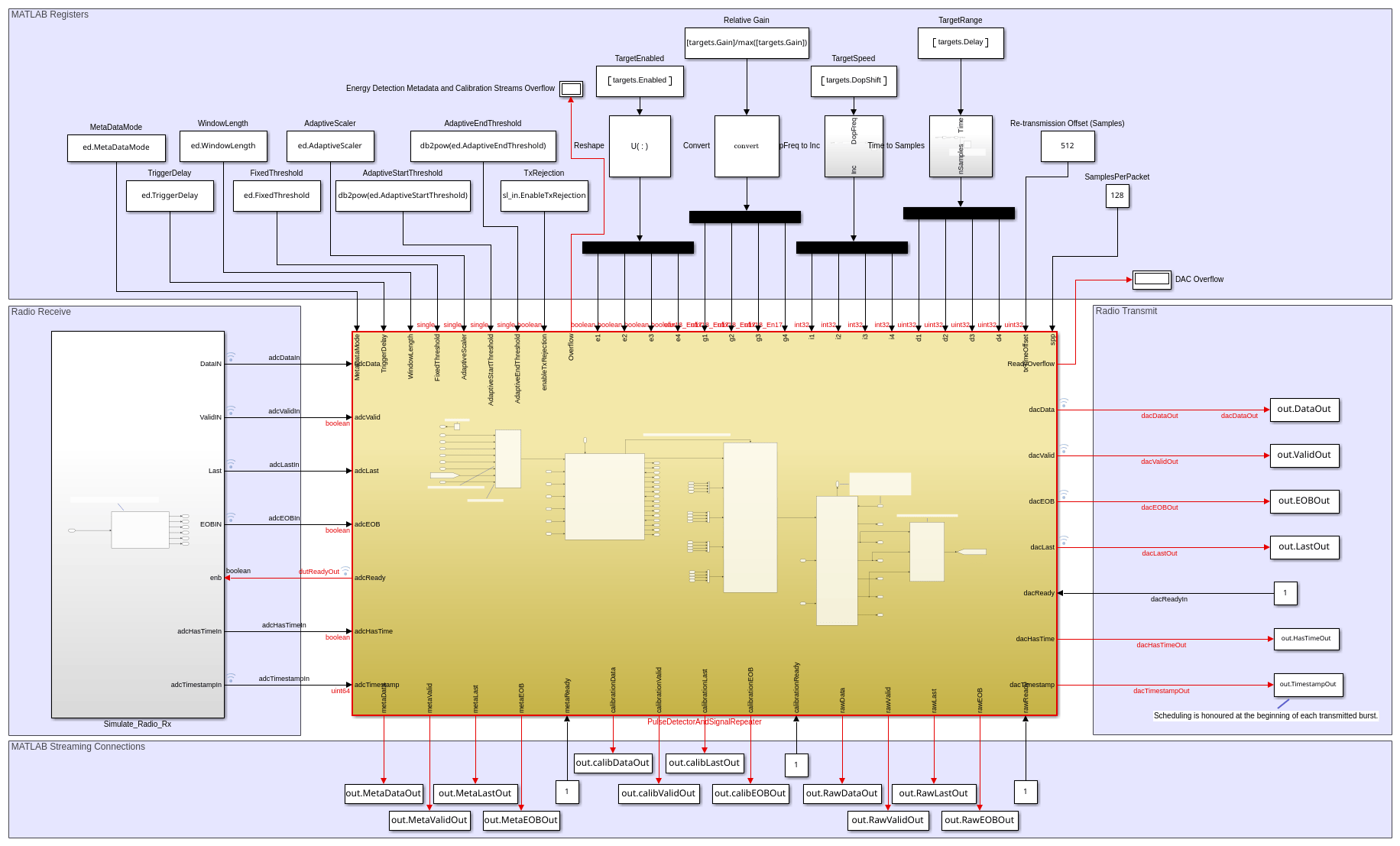
The top-level structure of the model includes the PulseDetectorAndSignalRepeater subsystem, which is the DUT. In addition, it contains subsystems and blocks that generate input data and save output data for simulating the behavior of the DUT model.
Open the PulseDetectorAndSignalRepeater subsystem.
open_system('wtPulseDetectionAndRepetitionSL/PulseDetectorAndSignalRepeater');
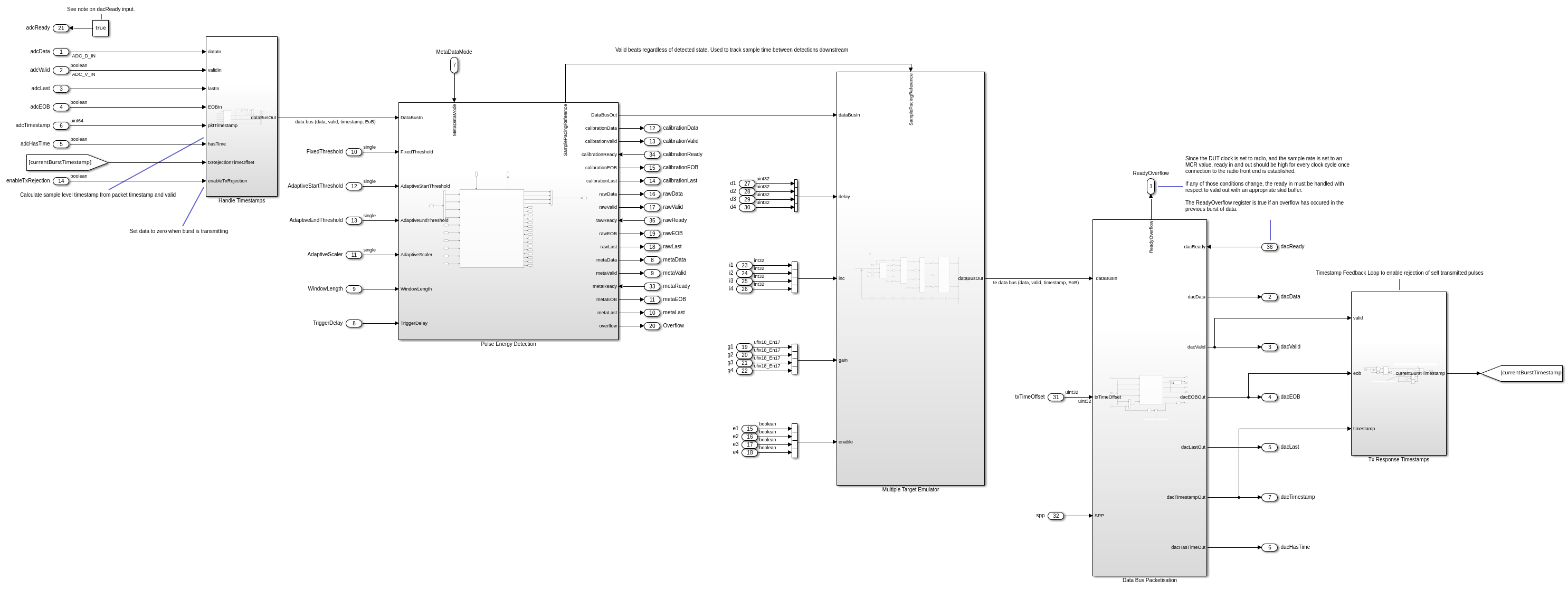
Data flows through these blocks and subsystems:
The
Handle Timestampssubsystem depacketizes the incoming data stream from the radio and optionally zeros data during transmission to prevent self-interference.The
Pulse Energy Detectionsubsystem detects the presence of pulses in the received data using an energy-based adaptive threshold.The
Multiple Target Emulatorsubsystem emulates the response of up to four targets by applying variable time delay, frequency shift, and attenuation to the detected pulses.The
Tx Response Timestampssubsystem tracks the timestamp of the current received burst for scheduling the retransmission.The
Data Bus Packetisationsubsystem implements the signaling for the streaming interface output.
Handle Timestamps Subsystem
Open the Handle Timestamps subsystem.
open_system('wtPulseDetectionAndRepetitionSL/PulseDetectorAndSignalRepeater/Handle Timestamps');
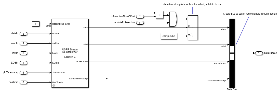
This subsystem performs two functions:
USRP stream depacketization - Extracts data, valid, end-of-burst, and sample timestamp signals from the incoming AXI streaming interface.
Transmit rejection - When transmit rejection is enabled, the subsystem zeros the data output when the sample timestamp is less than the transmit rejection time offset. This behavior prevents the algorithm from processing its own transmitted signal which avoids false detections.
Pulse Energy Detection Subsystem
Open the Pulse Energy Detection subsystem.
open_system('wtPulseDetectionAndRepetitionSL/PulseDetectorAndSignalRepeater/Pulse Energy Detection');
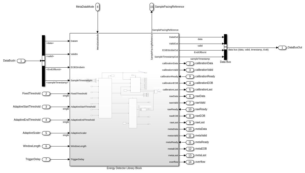
This subsystem detects the presence of radar pulses using an Energy Detector helper block from the Wireless Testbench targeting library. The energy detector operates as follows:
A sliding window computes the short-term energy of the received signal.
The detector uses both a fixed minimum energy threshold and an adaptive threshold based on the ratio of the current energy to the recent energy history.
When both thresholds are exceeded, a detection is triggered after a configurable trigger delay.
The detector outputs the detected pulse data along with calibration and metadata streams for debugging and tuning the threshold parameters.
The key parameters that control detection behavior are:
FixedThreshold- Minimum energy level required for detection.AdaptiveStartThreshold- Energy ratio (in dB) above the background that indicates the start of a pulse.AdaptiveEndThreshold- Energy ratio (in dB) that indicates the end of a pulse.WindowLength- Number of samples in the energy averaging window.TriggerDelay- Number of samples to delay the trigger point, allowing capture of the pulse rising edge.
Multiple Target Emulator Subsystem
The Multiple Target Emulator subsystem is the same subsystem that is used in the Radar Target Emulation on NI USRP Radio example. Open the subsystem.
open_system('wtPulseDetectionAndRepetitionSL/PulseDetectorAndSignalRepeater/Multiple Target Emulator');
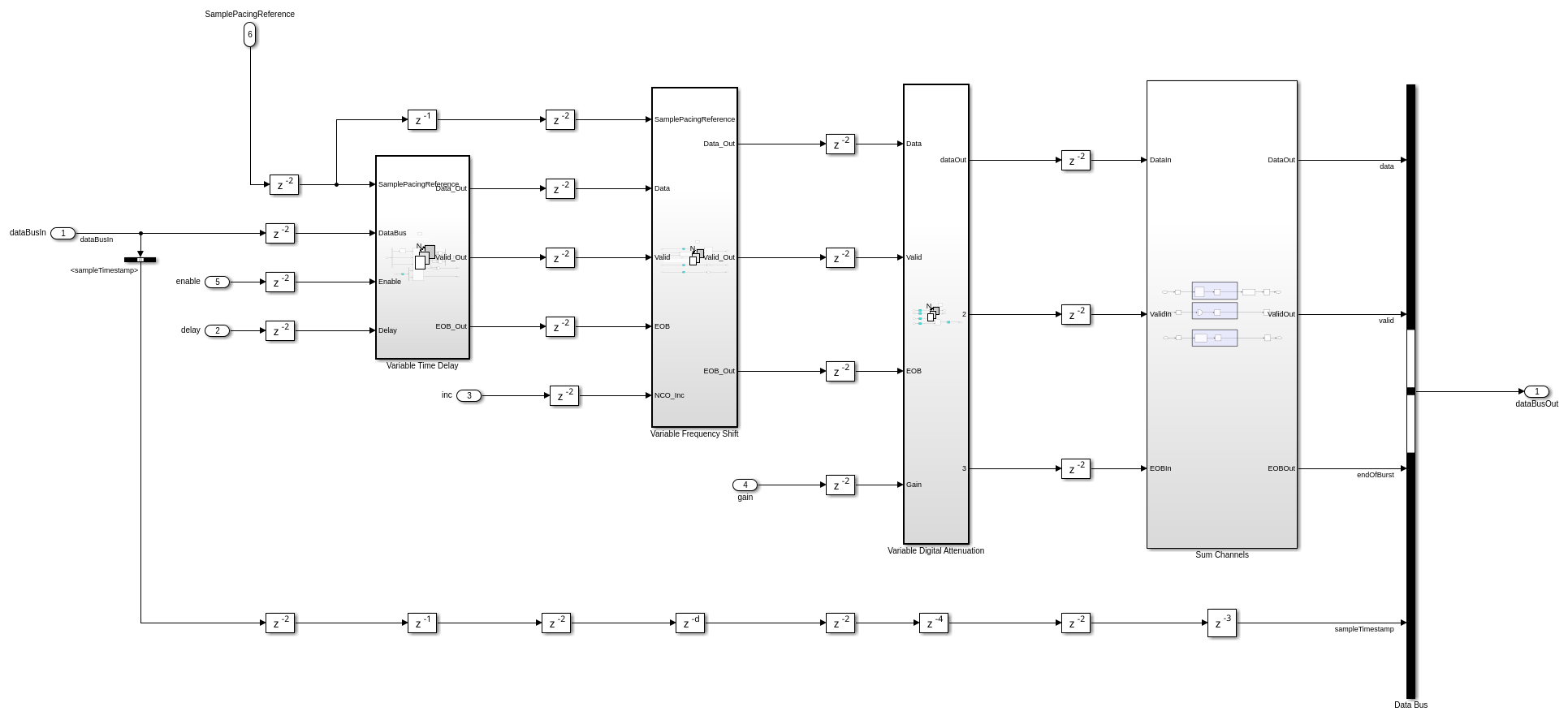
This subsystem emulates the response for four different targets by applying a variable time delay, variable frequency shift, and variable attenuation according to the enable, delay, inc, and gain input ports. The operation is as follows:
When enable is true, the detected pulse data is provided to the variable time delay.
The variable time delay buffers the input samples in memory for the number of samples specified by the delay port.
The delayed data is multiplied by the output of a numerically controlled oscillator (NCO) to achieve a variable frequency shift. The NCO is controlled by the inc port value.
The delayed and shifted data is multiplied by the gain port value to achieve a variable attenuation.
The
Sum Channelssubsystem combines the responses from the four targets into a single data stream.
Data Bus Packetization Subsystem
Open the Data Bus Packetisation subsystem.
open_system('wtPulseDetectionAndRepetitionSL/PulseDetectorAndSignalRepeater/Data Bus Packetisation');
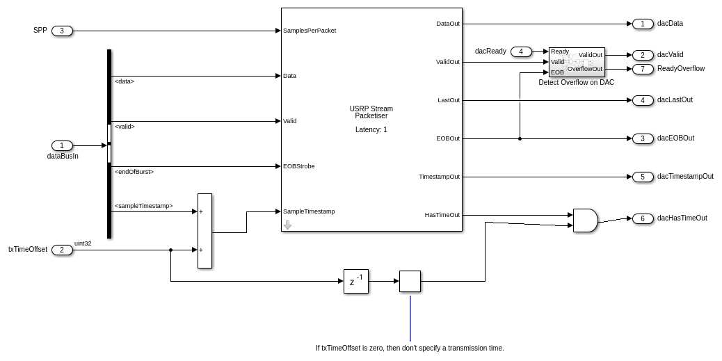
This subsystem implements the last, EOB, has time, and timestamp signals for the output stream to the radio DAC.
The SPP input port defines the samples per packet, which is the number of valid samples between assertions of the last signal. You can reduce round-trip latency of the pulse detector by specifying a smaller value for the SPP write register from MATLAB.
The txTimeOffset input sets the scheduled retransmission time as an offset from the received timestamp. If the txTimeOffset input value is set to zero, the has time signal is set low, specifying that the transmission should be scheduled as soon as possible. Specifying a nonzero value allows for precise sample-level control of the round-trip latency inside the FPGA.
Simulate Design
Verify the design by simulating the model. Set up the simulation parameters using the helperPulseDetectionAndRepetitionSetup function. This function configures the energy detector, target emulator, and simulated radar waveform parameters.
[sl_in, ed, targets] = helperPulseDetectionAndRepetitionSetup();
Add a small noise floor to the test signal to prevent divide-by-zero in the energy ratio calculation and to better represent a real RF environment.
sl_in.testSignal = reinterpretcast(sl_in.testSignal,numerictype(fixdt(1,16,15)));
sl_in.testSignal = fi(awgn(double(sl_in.testSignal),10,'measured'),fixdt(1,16,15));
sl_in.testSignal = reinterpretcast(sl_in.testSignal,numerictype('int16'));
The setup function creates four targets with different ranges and speeds. Display the target parameters.
for t = 1:numel(targets)
    fprintf('Target %d: Range = %.1f km, Speed = %.1f m/s, Enabled = %d\n', ...
        t, targets(t).Range/1e3, targets(t).Speed, targets(t).Enabled);
end
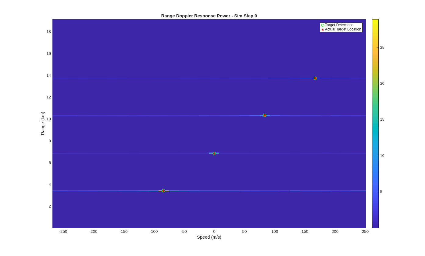
Target 1: Range = 3.4 km, Speed = -80.0 m/s, Enabled = 1
Target 2: Range = 6.9 km, Speed = 0.0 m/s, Enabled = 1
Target 3: Range = 10.3 km, Speed = 80.0 m/s, Enabled = 1
Target 4: Range = 13.8 km, Speed = 160.0 m/s, Enabled = 1
The hEnergyDetector helper object defines the operation of the energy detection algorithm and provides methods for tuning and calibration. Set the MetaDataMode property according to which metadata and calibration signals you want to be returned. * Set 0 to stream only the three word pulse description metadata. * Set 1 to also stream all the calibration signals for detector tuning. * Set 2 to only stream calibration signals while the detector is triggered. Use this setting to examine the IQ samples of each detection.
Set the MetaDataMode property to 1 so that you can plot the behavior of the detector after simulation.
ed.MetaDataMode = 1;
Simulate the model in rapid accelerator mode.
out = sim("wtPulseDetectionAndRepetitionSL.slx",SimulationMode="rapid-accelerator");
### Skipped unpacking from Simulink cache file "wtPulseDetectionAndRepetitionSL.slxc" because the relevant build artifacts on disk are up to date.
### Searching for referenced models in model 'wtPulseDetectionAndRepetitionSL'.
### Total of 1 models to build.
### Starting top model simulation target build for: wtPulseDetectionAndRepetitionSL
### Build folder for generated code: /home/user/Documents/MATLAB/ExampleManager/user.Bdoc.j3277699.ExampleSubmit/wt-ex10491246/slprj/raccel/wtPulseDetectionAndRepetitionSL
### Skipping code compilation for model "wtPulseDetectionAndRepetitionSL".

Build Summary

0 of 1 models built (1 models already up to date)
Build duration: 0h 0m 21.102s
Analyze Pulse Detection Results
The energy detector outputs three auxiliary data streams in addition to the main repeated signal:
Metadata - Contains a summary of each detected pulse including the pulse length, peak energy, and timestamp. Each pulse generates three metadata words.
Calibration - Contains the threshold signals used by the detection algorithm, including the energy output, energy delta, and trigger decision at every sample. Use this stream to tune the detection parameters.
Raw - Contains the unprocessed received IQ data aligned with the calibration stream for visual comparison.
Extract the valid samples from each stream.
calibData = out.calibDataOut(out.calibValidOut);
metaData = out.MetaDataOut(out.MetaValidOut);
rawData = out.RawDataOut(out.RawValidOut);
Process the metadata stream to extract pulse detection information. The processMetaDataStream function decodes the bit-packed metadata words into pulse length, peak energy, and timestamp for each detected pulse.
[pulseLength, pulsePeakEnergy, ~, pulseTimestamp] = ...
    processMetaDataStream(ed, metaData, sl_in.Fs);
Display the detected pulses in a table. Verify that the detector finds one pulse per PRI with consistent pulse lengths and uniform spacing that matches the configured pulse repetition interval.
pulseTable = table((1:numel(pulseLength))', ...
    double(pulseLength), ...
    double(pulsePeakEnergy), ...
    pulseTimestamp*1e3, ...
    VariableNames=["Pulse","Length (samples)","Peak Energy","Timestamp (ms)"])
pulseTable =

  32×4 table

    Pulse    Length (samples)    Peak Energy    Timestamp (ms)
    _____    ________________    ___________    ______________

      1             39             8.0547          0.000424
      2             39             8.0469           0.14042
      3             39             8.0156           0.28042
      4             39             8.0234           0.42042
      5             39             8.0469           0.56042
      6             39             8.0391           0.70042
      7             39             8.0234           0.84042
      8             39             7.9922           0.98042
      9             39             6.9766            1.1204
     10             39             8.0156            1.2604
     11             39             8.0391            1.4004
     12             39             8.0391            1.5404
     13             39             8.0156            1.6804
     14             39                  8            1.8204
     15             39             8.0312            1.9604
     16             39             8.0078            2.1004
     17             39             7.9883            2.2404
     18             39             7.9922            2.3804
     19             39             8.0234            2.5204
     20             39             8.0234            2.6604
     21             39             8.0391            2.8004
     22             39             8.0312            2.9404
     23             39             8.0391            3.0804
     24             39             8.0391            3.2204
     25             39             8.0234            3.3604
     26             39             8.0156            3.5004
     27             39             7.9922            3.6404
     28             39             8.0625            3.7804
     29             39             8.0156            3.9204
     30             39             8.0391            4.0604
     31             39             8.0156            4.2004
     32             39             7.9648            4.3404
Verify that the number of detected pulses matches the expected CPI length and that the pulse spacing is consistent.
fprintf('Expected pulses (CPI length): %d\n', sl_in.CPILength);
fprintf('Detected pulses: %d\n', numel(pulseLength));
fprintf('Mean pulse spacing: %.4f ms (expected PRI: %.4f ms)\n', ...
    mean(diff(pulseTimestamp))*1e3, 1/sl_in.PRF*1e3);
Expected pulses (CPI length): 32
Detected pulses: 32
Mean pulse spacing: 0.1400 ms (expected PRI: 0.1400 ms)
Visualize Energy Detection Threshold
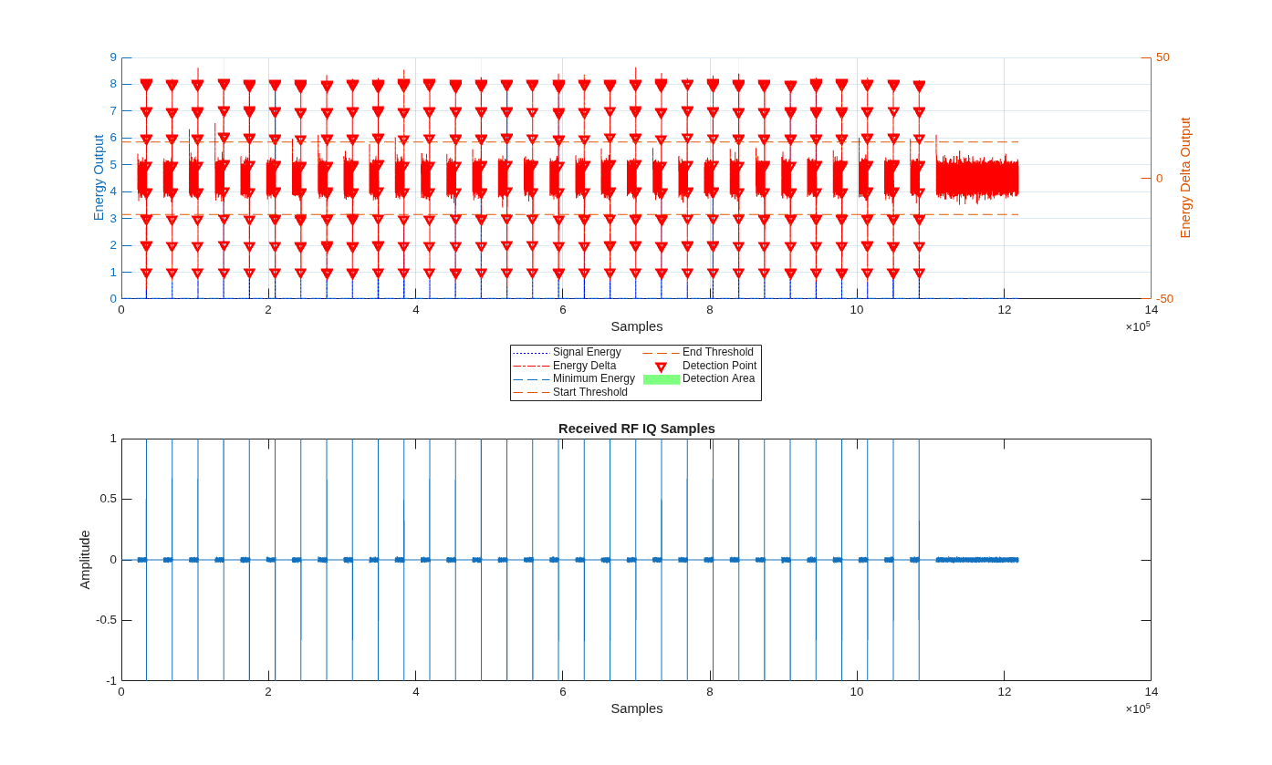
Plot the calibration signals to visualize how the energy detector identifies pulses. The upper plot shows the signal energy and adaptive energy delta along with their respective thresholds. Green shaded regions indicate where the detector has triggered. The lower plot shows the corresponding raw IQ data.
plotThreshold(ed, metaData, calibData, rawData, sl_in.Fs);
To see how the energy detector uses thresholds to detect a signal, zoom in on a single pulse.
calval = calibData(1024-ed.TriggerDelay:end-ed.TriggerDelay);
detectionVector = logical(bitshift(calval, -31));
pulseStarts = find(diff([false; detectionVector]) == 1);
pulseEnds = find(diff([detectionVector; false]) == -1);
pulseWidth = pulseEnds(2) - pulseStarts(2);
margin = pulseWidth/2;
xlim([pulseStarts(2)-margin pulseEnds(2)+margin]);
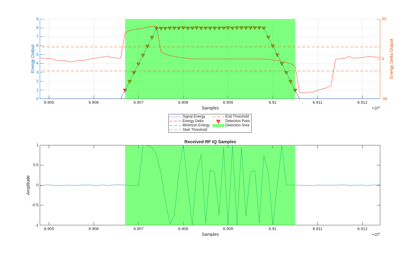
The energy detector uses a dual-threshold approach:
The fixed threshold sets an absolute minimum energy level, which prevents false triggers from noise.
The adaptive start threshold detects the rising edge of a pulse by comparing the current energy to the recent background. A positive value in dB means the energy must be this many dB above the background to trigger.
The adaptive end threshold detects the end of a pulse by identifying when the energy drops below the background level.
The trigger delay shifts the detection window backwards to capture the pulse rising edge, that would otherwise be missed.
Display the current energy detector configuration.
fprintf('Energy Detector Configuration:\n');
fprintf('  Fixed Threshold:          %.3f\n', ed.FixedThreshold);
fprintf('  Adaptive Start Threshold: %+.0f dB\n', ed.AdaptiveStartThreshold);
fprintf('  Adaptive End Threshold:   %+.0f dB\n', ed.AdaptiveEndThreshold);
fprintf('  Window Length:            %d samples\n', ed.WindowLength);
fprintf('  Trigger Delay:            %d samples\n', ed.TriggerDelay);
Energy Detector Configuration:
  Fixed Threshold:          0.030
  Adaptive Start Threshold: +15 dB
  Adaptive End Threshold:   -15 dB
  Window Length:            8 samples
  Trigger Delay:            4 samples
On hardware, use the testCalibration function of the hEnergyDetector helper object to capture these signals from the FPGA and iteratively tune the thresholds for the specific RF environment.
Plot Range-Doppler Response
Measure the internal latency of the DUT. On hardware, incorporate this delay into the set target delay to achieve real-time performance.
internalLatency = find(out.ValidOut,1) - sl_in.InitialZeroPadding;
disp("Measured internal latency is: "+string(internalLatency)+" clock cycles.")
Measured internal latency is: 116 clock cycles.
Create a range-Doppler response object for processing data.
rdResponse = phased.RangeDopplerResponse(...
    'DopplerFFTLengthSource','Property', ...
    'DopplerFFTLength',sl_in.VelDimLen, ...
    'PRFSource','Property', 'PRF',sl_in.PRF,...
    'SampleRate',sl_in.Fs,'DopplerOutput','Speed', ...
    'OperatingFrequency',sl_in.Fc);
Create a two-dimensional CFAR detector object for detection generation.
cfar = phased.CFARDetector2D(GuardBandSize=[25 1],...
    TrainingBandSize=[10 1],...
    ProbabilityFalseAlarm=1e-4);
Process the simulation output data and plot the range-Doppler response using the helperPlotRepeatedSignal function. The plot shows the detected targets overlaid with their actual locations, which verifies that the pulse detection and repetition algorithm correctly emulates multiple targets.
fig = figure;
ax = axes(fig);
data = out.DataOut(sl_in.InitialZeroPadding+internalLatency+1:end);
helperPlotRepeatedSignal(data,sl_in,targets,rdResponse,cfar,0,ax);
Configure IP Core
When you are satisfied with the simulated behavior of the model, you can proceed to integrate your design into a custom IP core by generating HDL code and mapping the model inputs and outputs to the hardware interfaces.
First, use the hdlsetuptoolpath (HDL Coder) function to set up the
tool chain. Specify the path to your Vivado® bin directory. For more information, see Set Up Third-Party Tools.
hdlsetuptoolpath('ToolName','Xilinx Vivado', ...
    'ToolPath','/opt/Xilinx/Vivado/2021.1/bin');
From the Apps tab in the Simulink Toolstrip, select HDL Coder. Then open the HDL Code tab.
Configure Output Options
To prepare the model for IP core generation, on the HDL Code tab, configure the output options:
Ensure the
PulseDetectorAndSignalRepeatersubsystem is pinned in the Code for option. To pin this selection, select thePulseDetectorAndSignalRepeatersubsystem in the Simulink model and click the pin icon.Select IP Core as the Output > IP Core option.

Configure HDL Code Generation Settings
Open the Configuration Parameters dialog box by clicking Settings in the HDL Code tab.
In the HDL Code Generation pane, ensure that Language is set to Verilog. By default, HDL Coder generates the Verilog® files in the hdlsrc folder. You can select an alternative location. If you make any changes, click Apply.

On the Target pane, configure these settings:
Under Workflow Settings, select the
IP Core
                        Generation
workflow. To set Project Folder, click Browse and select a target location for saving the generated project files. If you do not specify a project folder, the software saves the generated project files in the working directory.Under Tool and Device Settings, select your radio from the Target Platform list. This example uses a USRP N320 radio. If you are using a different radio, adjust the reference design parameters to match your hardware.
Under Reference Design Settings, set Reference Design to
HG: 10GigE.Set the reference design parameters to these values:
Number of Input Streams — Set to
1because the DUT receives one data input stream from the radio antenna.Number of Output Streams — Set to
4because the DUT produces four data output streams: one for transmission from the target emulator, and three for data from the energy detector to the host (pulse metadata, calibration data, and raw IQ data).Sample Rate (S/s) — Set to the maximum sample rate supported by your radio. This example uses a USRP N320 radio and a sample rate of 250 MS/s, which corresponds to the maximum supported master clock rate (MCR), 250 MHz. For more information about supported values on your radio, see Determine Radio Device Capabilities.
Reference Design Optimization — Set to
High. This optimization level creates static connections between the DUT and the radio antennas, removing the digital down-conversion (DDC) and digital up-conversion (DUC) logic. This reduces latency by enabling a smaller number of samples per packet on the streaming interface. This setting also reduces FPGA resource utilization, which is required on some radios to meet timing constraints.DUT Clock Source — Set to
Radio. The DUT is clocked at the MCR used by the radio to achieve the specified sample rate.Stream Port FIFO Length (Samples) — Set to
Auto. This setting automatically calculates the buffer length for each DUT input and output data streaming port.Register Port FIFO Length (Samples) — Set to
Auto. This setting automatically calculates the buffer length for each DUT register port.
Under Objectives Settings, because the DUT Clock Source is set to
Radio, the Target Frequency is fixed at the highest supported MCR of the radio.
Click Apply.

On the Optimization pane, select Distributed pipelining.

To apply these settings and close the Configuration Parameters window, click OK.
For more information, see Configure HDL Code Generation Settings.
Map Target Interfaces
On the HDL Code tab, click Target Interface
to open the Interface Mapping table in the IP Core editor. To
populate the table with your user logic, click the Reload IP core settings button:  .
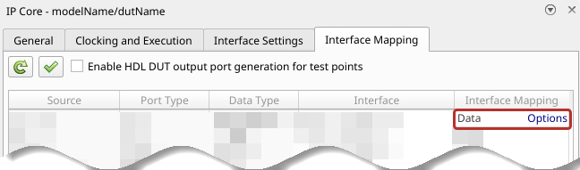
The Source, Port Type, and Data Type columns are populated based on the Simulink model. In this example, the Interface column is prepopulated because the model is saved with the interface mapping already assigned.
The energy detector configuration ports (
MetaDataMode,TriggerDelay,WindowLength,FixedThreshold,AdaptiveScaler,AdaptiveStartThreshold,AdaptiveEndThreshold,enableTxRejection) and target emulator channel ports (e1–e4,g1–g4,i1–i4,d1–d4,txTimeOffset,spp) map toWrite Registerinterfaces.The
adcData,adcValid,adcLast,adcEOB,adcHasTime,adcTimestamp, andadcReadyports map to aStream Port Input0interface. This stream is the incoming samples from the DUT input antenna on the radio.The
dacData,dacValid,dacLast,dacEOB,dacHasTime,dacTimestamp, anddacReadyports map to aStream Port Output0interface. This stream sends the retransmitted pulses to the DUT output antenna on the radio.The
metaData,metaValid,metaLast,metaEOB, andmetaReadyports map to aStream Port Output1interface. This stream sends pulse metadata to the host computer.The
calibrationData,calibrationValid,calibrationLast,calibrationEOB, andcalibrationReadyports map to aStream Port Output2interface. This stream optionally sends calibration data to the host computer.The
rawData,rawValid,rawLast,rawEOB, andrawReadyports map to aStream Port Output3interface. This stream optionally sends raw IQ samples to the host computer.The
ReadyOverflowandOverflowports map toRead Registerinterfaces. These registers indicate overflows on the transmitter stream and energy detector streams respectively.
The Interface Mapping column is populated automatically based on the signal names in the model. If the mapping is incorrect, manually adjust the Interface Mapping column.
To set the interface options for the streaming interfaces, open the Set Interface Options window by clicking Options in the far right of the table.
For the
adcDatainterface options, select a receive antenna as the source connection. The DUT receives input samples from this antenna on the radio. Set the stream buffer size to32768, which is the default setting.For the
dacDatainterface options, select a transmit antenna as the sink connection. The DUT sends retransmitted pulses to this antenna on the radio.Note
Because the reference design optimization is set to
High, once mapped, the antenna selections are fixed and cannot be changed at run time. The design requires independent transmit and receive paths, so choose antennas that do not form an FPGA loopback pair. For example, for a USRP N320 radio, select the first enumerated antenna,RF0:RX2for theadcDatastream, and the second enumerated transmit antenna,RF1:TX/RX, for thedacDatastream. For more information, see theLoopbackModeproperty description.For the
metaDatainterface options, selectHostas the sink connection. The energy detector streams pulse metadata to the host computer for logging and analysis. The data rate is low, so buffering is not required.For the
calibrationDataandrawDatainterface options, selectPL DDR Bufferas the sink connection. These streams use the PL DDR memory to buffer calibration signals and raw IQ samples for host read back.Note
If your radio is a USRP E320 or X310, the two available PL DDR buffer connections are required for the transmit and capture antennas used to test the deployed design. Connect the
calibrationDataandrawDatastreams directly to the host by selectingHostas the sink connection. The data rate you can achieve on these streams without overflows depends on the network connection.
When you have populated the table, validate the interface mapping by clicking the
Validate IP core settings button:  .
For more information, see Map Target Interfaces.
Generate and Load Bitstream
To generate a bitstream from the configured IP core, select Build Bitstream > Deployment Settings.

Ensure that the Run build process externally option is selected. This setting is the default and it ensures that the bitstream build executes in an external shell, which allows you to continue using MATLAB while building the FPGA image.
In the Program Target Device settings, set the IP address. The default is
192.168.10.2. If your radio has a different IP address, update this value.

Click Build Bitstream to create a Vivado IP core project and build the bitstream. After the basic project checks
complete, the Diagnostic Viewer displays a Build Bitstream Successful
message along with warning messages. However, you must wait until the external shell
displays a successful bitstream build before moving to the next step. Closing the external
shell before this time terminates the build.
The bitstream for this project generates with the name n3xx.bit and
is located in the build_N320_HG/build_N320_HG folder of the working
directory after a successful bitstream build. If you are using a different radio, the name
and location reflect your radio.
To load the bitstream onto the device now, select Build Bitstream > Program Target Device. Alternatively, you can load the bitstream later by using the
programFPGA function in the generated host interface script.
For more information, see Generate Bitstream and Program FPGA.
Generate Host Interface Scripts
To generate MATLAB scripts that enable you to connect to and run your deployed design on your radio, in the HDL Code tab, click Host Interface Script. This step generates two scripts in your working directory based on the target interface mapping that you configured for your IP core.
gs_wtPulseDetectionAndRepetitionSL_interface.m— Host interface script that creates anfpgaobject for interfacing with your DUT running on the FPGA from MATLAB. The script contains code that connects to your hardware and programs the FPGA and code samples to get you started with running the algorithm on your radio. For more information, see Interface Script File.gs_wtPulseDetectionAndRepetitionSL_setup.m— Setup function that configures thefpgaobject with the hardware interfaces and ports from your DUT algorithm. The function contains DUT port objects that have the port name, direction, data type, and interface mapping information, which it maps to the corresponding interfaces. For more information, see Setup Function File.Note
The number of samples per host-side
readPortorwritePortoperation, specified in theFrameSizename-value argument of theaddRFNoCStreamInterfacefunction, is set by default to 1e5. To change this value or the value of theTimeoutname-value argument, edit the setup function file.
Verify Pulse Detection and Signal Repetition Algorithm Using MATLAB
To verify the pulse detection and signal repetition algorithm running on your radio, use this script to run a target scenario on hardware.
To test the algorithm on a single radio, the script follows these steps:
Set up and configure the radio with the generated bitstream and interfaces.
Configure additional radio antennas for transmit and capture from the host.
Configure the energy detector and target emulation DUT with the default scenario parameters.
Schedule the transmission of a radar pulse train.
Schedule the streaming of IQ samples from the air into the onboard memory.
Analyze the pulse detection results and plot the range-Doppler response for the samples captured by the host.
Open Live Script
You can open this live script in MATLAB from the example working directory and use it interactively. In the Files panel, navigate to your example working directory and open VerifyPulseDetectionAndRepetitionAlgorithmUsingMATLABExample.m.
Set Up Radio
Select Radio
To retrieve your saved radio setup configurations, call the radioConfigurations function. The function returns all available radio setup configurations that you saved using the Radio Setup wizard.
savedRadioConfigurations = radioConfigurations;
To update the menu with your saved radio setup configuration names, click Update. Then select the radio to use with this example.
savedRadioConfigurationNames = string({savedRadioConfigurations.Name});
radioConfig =  savedRadioConfigurationNames(1)
 ;
Evaluate the transmit and receive antennas available on your radio device. You select transmit and capture antennas from the available options later in the script.
availableReceiveAntennas = hCaptureAntennas(radioConfig);
availableTransmitAntennas = hTransmitAntennas(radioConfig);
To connect to your radio hardware, create a radio object and a usrp System object with the specified radio.
radio = radioConfigurations(radioConfig);
device = usrp(radio);
Program FPGA
If you have not yet programmed your device with the bitstream, select the program bitstream option. Update the code with your bitstream and hand-off information files. You can find these in the generated host interface script, gs_wtPulseDetectionAndRepetitionSL_interface. If your radio device is a USRP X310, you only require a bitstream file to program the FPGA.
programBitstream =false; if(programBitstream) programFPGA(device, ... "build_N320_HG/build-N320_HG/n3xx.bit", ... % replace with your .bit file "build_N320_HG/build/usrp_n320_fpga_HG.dts"); % replace with your .dts file end
To configure the DUT interfaces according to the hand-off information file, use the describeFPGA function. This function also sets the values for the SampleRate, DUTInputAntennas, and DUTOutputAntennas properties based on the selections you made in Simulink.
describeFPGA(device,"wtPulseDetectionAndRepetitionSL_wthandoffinfo.mat");Configure Device
Configure your usrp System object to loop back the waveform through the target emulator. You can loop back over the air or directly on the FPGA.
Set the LoopbackMode property to FPGA to loop back each transmit antenna to an associated receive antenna on the FPGA. Alternatively, you can select Disabled to transmit and receive data over the air. FPGA loopback is not available on radios that have no transmit antennas.
device.LoopbackMode =  "FPGA";
Because the bitstream is generated with Reference Design Optimization set to High, the radio antennas connected to the DUT are fixed to the options you configured in the Interface Mapping table in Simulink. To use FPGA loopback, your DUT must be configured with an input and output antenna connection that is a valid loopback antenna pair. For details, see the table in the LoopbackMode property description.
Specify a transmit antenna and a capture antenna to exercise the target emulation DUT from MATLAB. Because the bitstream is generated with the Reference Design Optimization parameter set to High, there is a single transmit and capture antenna available.
device.TransmitAntennas = availableTransmitAntennas(1);
device.CaptureAntennas = availableReceiveAntennas(2);
If you are transmitting and receiving over the air using antennas, specify the center frequency and radio gains for each antenna. If FPGA loopback is enabled, these properties have no effect.
Specify the center frequency for the transmit and receive antennas. To loop back over the air, ensure the transmit and receive center frequencies are equal.
centerFrequency = 2e9;
device.ReceiveCenterFrequency = centerFrequency;
device.TransmitCenterFrequency = centerFrequency;
Specify the RF gain for the target emulator input and output according to your RF setup and hardware. The output gain is a reference corresponding to the maximum output power of the target emulator.
targetEmulatorInputRadioGain =30; targetEmulatorOutputRadioGainReference =
30;
Specify the radio gains for the MATLAB transmit and capture antennas. Set the value according to your RF setup and hardware.
mlCaptureRadioGain =30; mlTransmitRadioGain =
30;
Set the radio gain values for each antenna using the usrp System object.
device.ReceiveRadioGain = [targetEmulatorInputRadioGain,mlCaptureRadioGain];
device.TransmitRadioGain = [targetEmulatorOutputRadioGainReference,mlTransmitRadioGain];
Create and Set Up fpga Object
Create an fpga object to interface with the DUT ports you designed in Simulink.
dut = fpga(device);
Set up the fpga object using the generated setup function. The function maps the stream interfaces and register ports.
gs_wtPulseDetectionAndRepetitionSL_setup(dut);
The generated setup function sets a frame size for each streaming interface connected to MATLAB. This example uses the default value of 1e5.
streamPortFrameSizes = table(string.empty,[],VariableNames = ["PortName","FrameSize"]);
for port = ["metaData","calibrationData","rawData"] % Stream ports on DUT
    idx = find(cellfun(@(c) any(strcmp(c,port)), {dut.Interfaces.OutputPorts}));
    streamPortFrameSizes(end+1,:) = {port, dut.Interfaces(idx).FrameSize};
end
streamPortFrameSizes
streamPortFrameSizes = 3×2 table
        PortName         FrameSize
    _________________    _________

    "metaData"             1e+05
    "calibrationData"      1e+05
    "rawData"              1e+05

	Get insights using Copilot
Optimize Round-Trip Latency
To optimize the round-trip latency of the pulse detector, tune the samples per streaming packet and the overall scheduled re-transmission time offset.
The samples per packet (SPP) input defines the number of valid samples between assertions of the last signal. If the SPP input is zero, which is the default value of the register on the hardware, the DUT uses an SPP of 256. A lower SPP value reduces packet latency, but increases overhead on the streaming connection, which reduces maximum throughput. If the SPP is too low, overflows occur.
The txTimeOffset input sets the scheduled re-transmission time as an offset from the received timestamp. If txTimeOffset is zero, the radio schedules the transmission as soon as possible. A nonzero value provides precise sample-level control of the round-trip latency inside the FPGA. If txTimeOffset is too short, the burst might arrive late at the radio front-end. If txTimeOffset is longer than the available buffers, overflows occur due to backpressure.
These values, SPP equal to 100 and reTxOffset set to 512, are tuned on a USRP N320 radio. You might need to tune these values for other radio hardware.
device.SamplesPerPacket = 100;
reTxOffset = 512;
Set Up Radar Scenario
Customize the simulation for your radio hardware by editing the helperPulseDetectionAndRepetitionSetup function. Run the setup helper function with the sample rate and center frequency for your radio hardware.
[sl_in, ed, targets] = helperPulseDetectionAndRepetitionSetup(device.SampleRate,device.ReceiveCenterFrequency);
Set Up usrp Object
To connect to the radio hardware, call setup on the device System object.
setup(device);
Reconnecting to radio. Radio time and GPIO configuration will be reset.
Configure Energy Detector
After connecting to the radio, configure the energy detector registers on the FPGA. The hEnergyDetector helper object manages the detection parameters and provides functions for writing them to the hardware and calibrating the thresholds.
Connect the energy detector helper object to the device and DUT.
connect(ed,device,dut);
The MetaDataMode property controls which auxiliary data streams the FPGA returns:
Set to 0 to stream only the three-word pulse description metadata.
Set to 1 to stream all calibration signals for detector tuning.
Set to 2 to stream calibration signals only while the detector is triggered.
To avoid overflow on the calibration and raw data streaming interfaces during the full pulse train capture, stream only the metadata. Set MetaDataMode to 0, which is the default value. Use the testCalibration function later to capture and visualize calibration signals with a shorter capture.
ed.MetaDataMode = 0;
write(ed);
Configure Transmit Waveform
Format the transmit waveform pulse train according to the slow time dimension length. Then scale as a 16-bit integer.
txPulseTrain = repmat( ...
    [sl_in.txSignal; zeros(sl_in.pulsePeriodSamples-length(sl_in.txSignal),1)], ...
    sl_in.VelDimLen, 1)*double(intmax("int16"));
captureLength = length(txPulseTrain);
When using FPGA loopback mode, add noise to the signal.
if strcmp(device.LoopbackMode,"FPGA")
    txPulseTrain = awgn(txPulseTrain,10,"measured");
end
Specify a scheduling offset. This is the number of seconds in the future the transmit and receive operations will start. The offset must be long enough to account for the loading of the transmit waveform into the PL DDR buffer before the transmission starts.
scheduleTimeOffset =  1;
Visualize Energy Detection Threshold
Use the testCalibration object function to capture the calibration signals and visualize the detection thresholds. This function sets the MetaDataMode property to 1, streams a short capture from the radio front-end, and reads the calibration and raw data streams. It checks for overflow, plots the threshold behavior, and restores the initial MetaDataMode value.
Flush any stale data from the metadata streaming interface before the main capture.
readPort(dut,"metaData");Schedule a new transmission so the energy detector has signal to detect during the calibration capture.
currentRadioTime = getRadioTime(radio);
scheduledTime = currentRadioTime + scheduleTimeOffset;
transmit(device,txPulseTrain,"once",StartTime=scheduledTime);
Use the testCalibration object function to capture and plot the threshold signals. Use a short capture length (a few PRIs) to avoid overflow on the calibration streaming interface, which has a limited frame buffer size.
calibrationCaptureSamples = sl_in.pulsePeriodSamples * 2;
[pulseLength,pulsePeakEnergy,pulseTimestampSamples]  = testCalibration(ed,calibrationCaptureSamples,StartTime=scheduledTime);
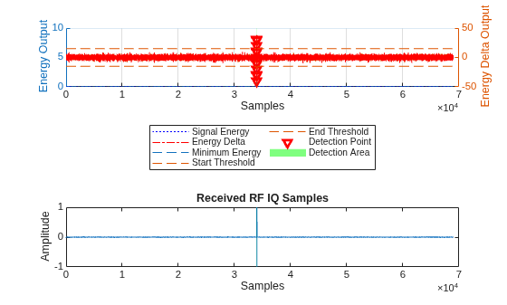
Zoom in on the most recent detected pulse to inspect the threshold crossing in detail. Convert the absolute pulse timestamp to a plot index by subtracting the capture start time.
if ~isempty(pulseTimestampSamples)
    startTimeSamples = uint64(scheduledTime * device.MCR);
    firstPulseIdx = double(pulseTimestampSamples(end) - startTimeSamples) - ed.SteadyStateOffset;
    margin = 20;
    calAxes = findobj(gcf,"Type","axes");
    xlim(calAxes(1), [max(1, firstPulseIdx - margin), firstPulseIdx + pulseLength(end)+margin]);
end
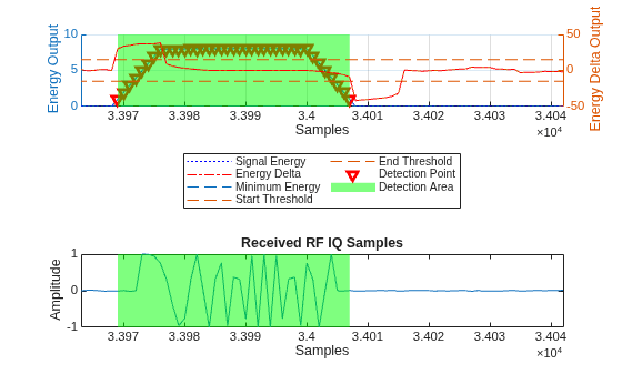
Iteratively tune the energy detector thresholds for your specific RF environment using the properties on the hEnergyDetector helper object. Use the write object function to update the FPGA registers, and then use the testCalibration object function to capture and plot the updated threshold behavior. Display the current energy detector configuration.
ed
ed =
  hEnergyDetector with properties:

            FixedThreshold: 0.0300
            AdaptiveScaler: 1
    AdaptiveStartThreshold: 15
      AdaptiveEndThreshold: -15
              TriggerDelay: 4
              WindowLength: 8
              MetaDataMode: 0
           MaxTriggerDelay: 63
Set Initial Target Emulator State
Use the writePort function to configure the register ports on the target emulator algorithm. The values come from the default target scenario state defined in the helperPulseDetectionAndRepetitionSetup function.
Specify the front-end delay so that it can be accounted for in the target delay. When using FPGA loopback mode, set this value to zero. If this is not accounted for when you transmit and receive the data over the air, there will be a small shift in the estimated ranges.
calibratedFrontEndDelay = 0;
Enable transmit rejection to prevent the algorithm from processing its own transmitted signal.
writePort(dut,"enableTxRejection",sl_in.EnableTxRejection);Select a reference gain which corresponds to the RF gain reference set on the DUT output antenna. Set to the maximum target gain to maximize use of the fixed-point range and minimize quantization effects.
maxGainReference = max([targets([targets.Enabled]).Gain]);
Update the register ports of the target emulator.
for target = 1:sl_in.TargetEmulator_NumChannels
    targetInc = targets(target).DopShift * (2^sl_in.TargetEmulator_NCO_accum_wl / sl_in.Fs);
    targetDelaySamples = nearest(abs(targets(target).Delay) * sl_in.Fs - reTxOffset - calibratedFrontEndDelay);
    writePort(dut,"e"+target,targets(target).Enabled);
    if targets(target).Enabled
        writePort(dut,"d"+target,targetDelaySamples);
        writePort(dut,"i"+target,targetInc);
        writePort(dut,"g"+target,maxGainReference/targets(target).Gain);
    end
end
writePort(dut,"spp",device.SamplesPerPacket);
writePort(dut,"txTimeOffset",reTxOffset);
Display the target parameters.
for t = 1:numel(targets)
    fprintf('Target %d: Range = %.1f km, Speed = %.1f m/s, Enabled = %d\n', ...
        t, targets(t).Range/1e3, targets(t).Speed, targets(t).Enabled);
end
Target 1: Range = 3.4 km, Speed = -80.0 m/s, Enabled = 1
Target 2: Range = 6.9 km, Speed = 0.0 m/s, Enabled = 1
Target 3: Range = 10.3 km, Speed = 80.0 m/s, Enabled = 1
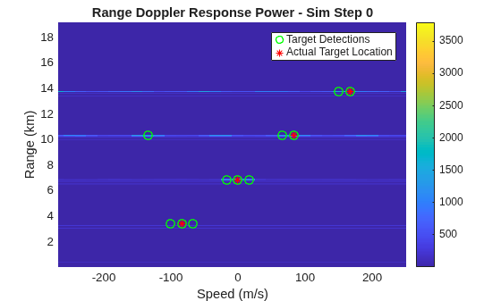
Target 4: Range = 13.8 km, Speed = 160.0 m/s, Enabled = 1
Verify DUT
Transmit the radar pulse train and capture the repeated signal to verify the pulse detection and target emulation behavior on hardware.
Flush any stale data from the metadata streaming interface before the main capture.
readPort(dut,"metaData");Schedule the transmit and receive operations to begin at the specified time offset.
currentRadioTime = getRadioTime(radio);
scheduledTime = currentRadioTime + scheduleTimeOffset;
Use the transmit function to schedule a single-shot transmission shortly after the scheduled time to allow the energy detector algorithm to reach a steady state.
steadyStateDelay = double(ed.WindowLength*2);
transmit(device,txPulseTrain,"once", ...
    StartTime=scheduledTime+steadyStateDelay/device.SampleRate);
Call the usrp System object directly to stream samples from the DUT input and capture antennas.
device(captureLength+steadyStateDelay, ...
    StartTime=scheduledTime, ...
    Background=false);
Use the capture function to retrieve the captured samples from the PL DDR buffer.
[capturedData,nSamps] = capture(device,captureLength+steadyStateDelay);
capturedData = capturedData(steadyStateDelay+1:nSamps,:);
Analyze Pulse Detection Results
When MetaDataMode is set to 0, the FPGA populates only the metadata stream. The metadata summarizes each detected pulse in terms of length, peak energy, and timestamp. Each pulse generates three metadata words.
Read the metadata streaming interface to retrieve the pulse detection results from the FPGA.
[metaData, numSamps_metaData, overflow_metaData] = readPort(dut,"metaData");Check for overflow on the metadata streaming interface.
if overflow_metaData
    warning("Overflow detected on the metadata streaming interface. Data was lost. Consider requesting fewer samples or selecting 'PL DDR Buffer' as the sink connection in the Simulink interface mapping table.")
end
Process the metadata stream to extract pulse detection information. The processMetaDataStream object function decodes the bit-packed metadata words into pulse length, peak energy, and timestamp for each detected pulse.
metaData = metaData(1:numSamps_metaData);
[pulseLength, pulsePeakEnergy, ~, pulseTimestamp] = ...
    processMetaDataStream(ed,metaData,device.MCR);
Display the detected pulses in a table. The detector should find one pulse per PRI, with consistent pulse lengths and a uniform spacing matching the configured pulse repetition interval (PRI). The pulse length measured depends on the energy detector thresholds and window length.
pulseTable = table((1:numel(pulseLength))', ...
    double(pulseLength), ...
    double(pulsePeakEnergy), ...
    pulseTimestamp*1e3, ...
    VariableNames=["Pulse","Length (samples)","Peak Energy","Timestamp (ms)"])
pulseTable = 32×4 table
    Pulse    Length (samples)    Peak Energy    Timestamp (ms)
    _____    ________________    ___________    ______________

      1             39             8.0312          9.6e-05
      2             39             8.0469            10369
      3             39             8.0312            10369
      4             39             6.9727            10369
      5             39             8.0156            10369
      6             39             8.0469            10369
      7             39             7.9727            10369
      8             39             7.9766            10369
      9             39             8.0234            10370
     10             39             8.0469            10370
     11             39             6.9883            10370
     12             39             8.0547            10370
     13             39             8.0078            10370
     14             39             8.0625            10370
     15             39             8.0703            10370
     16             39             8.0547            10371

	Get insights using Copilot
      ⋮
Verify that the number of detected pulses matches the expected coherent processing interval (CPI) length and that the pulse spacing is consistent.
fprintf('Expected pulses (CPI length): %d\n', sl_in.CPILength);Expected pulses (CPI length): 32
fprintf('Detected pulses: %d\n', numel(pulseLength));Detected pulses: 32
fprintf('Mean pulse spacing: %.4f ms (expected PRI: %.4f ms)\n', ...
    mean(diff(pulseTimestamp(2:end)))*1e3, 1/sl_in.PRF*1e3);
Mean pulse spacing: 0.1400 ms (expected PRI: 0.1400 ms)
Configure Detection
Create a phased.RangeDopplerResponse (Phased Array System Toolbox) object to analyze the received responses.
rdResponse = phased.RangeDopplerResponse(...
    DopplerFFTLengthSource="Property", ...
    DopplerFFTLength=sl_in.VelDimLen, ...
    PRFSource="Property",PRF=sl_in.PRF,...
    SampleRate=sl_in.Fs, ...
    DopplerOutput="Speed", ...
    DopplerWindow="Hamming", ...
    OperatingFrequency=sl_in.Fc);
Create a 2D constant false alarm rate (CFAR) detector object for detection generation. For optimal results, tune the parameters for your radio and setup.
cfar = phased.CFARDetector2D(GuardBandSize=[20 2], ...
    TrainingBandSize=[50 2],ProbabilityFalseAlarm=1e-6);
Plot Range-Doppler Response
Process the captured data and plot the range-Doppler response using the helperPlotRepeatedSignal function. The plot shows the detected targets overlaid with their actual locations, verifying that the pulse detection and repetition algorithm correctly emulates multiple targets on hardware.
fig = figure;
ax = axes(fig);
helperPlotRepeatedSignal(capturedData,sl_in,targets,rdResponse,cfar,0,ax);
Release Hardware Resources
Release the hardware resources.
release(dut);
release(device);
Conclusion
This example uses a pulse detection and signal repetition design with an energy detection stage that can identify and characterize pulses.
The example shows how to:
Deploy a pulse detection and signal repetition algorithm on the FPGA of an NI USRP radio.
Set the energy detector thresholds and target scenario parameters for your specific RF environment.
Monitor the detected pulses on the host computer and use the characterization data to decide when to enable the target emulation stage.
Retransmit emulated target responses and verify the correct behavior.
To test the design with real-world signals, set LoopbackMode to
Disabled and transmit and receive over the air. You can also use a
second radio as an external radar transmitter to exercise the deployed design with an
independent signal source.

