Wavelet Interval-Dependent Denoising

The example shows how to denoise a signal using interval-dependent thresholds.

In this example, we perform six trials to denoise the electrical signal nelec using these procedures:

Using one interval with the minimum threshold value: 4.5.
Using one interval with the maximum threshold value: 19.5.
Manually selecting three intervals and three thresholds, and using the wthresh function to threshold the coefficients.
Using the utthrset_cmd function to automatically find the intervals and the thresholds.
Using the cmddenoise function to perform all the processes automatically.
Using the cmddenoise function with additional parameters.

Denoising Using a Single Interval

Load the electrical consumption signal nelec.

load nelec.mat
sig = nelec;

Now we use the discrete wavelet analysis at level 5 with the sym4 wavelet. We set the thresholding type to 's' (soft).

wname = 'sym4';
level = 5;
sorh  = 's';

Denoise the signal using the function wdencmp with the threshold set at 4.5.

thr = 4.5;
[sigden_1,~,~,perf0,perfl2] = wdencmp('gbl',sig,wname,level,thr,sorh,1);
res = sig-sigden_1;
subplot(3,1,1)
plot(sig,'r') 
axis tight
title('Original Signal')
subplot(3,1,2)
plot(sigden_1,'b') 
axis tight
title('Denoised Signal')
subplot(3,1,3)
plot(res,'k') 
axis tight
title('Residual')

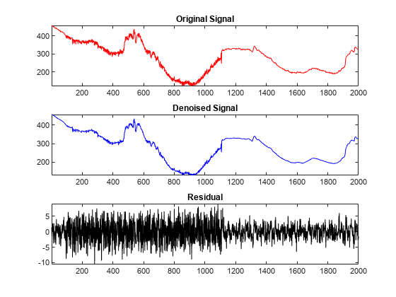
Figure contains 3 axes objects. Axes object 1 with title Original Signal contains an object of type line. Axes object 2 with title Denoised Signal contains an object of type line. Axes object 3 with title Residual contains an object of type line.

perf0,perfl2

perf0 = 
66.6995

perfl2 = 
99.9756

The obtained result is not good. The denoising is very efficient at the beginning and end of the signal, but between 100 and 1100 the noise is not removed. Note that the perf0 value gives the percentage of coefficients set to zero and the perfl2 value gives the percentage of preserved energy.

Now, we denoise the signal with a threshold of 19.5.

thr = 19.5;
[sigden_2,cxd,lxd,perf0,perfl2] = ...
    wdencmp('gbl',sig,wname,level,thr,sorh,1);
res = sig-sigden_2;
subplot(3,1,1)
plot(sig,'r')
axis tight
title('Original Signal')
subplot(3,1,2)
plot(sigden_2,'b')
axis tight
title('Denoised Signal')
subplot(3,1,3)
plot(res,'k')
axis tight
title('Residual')

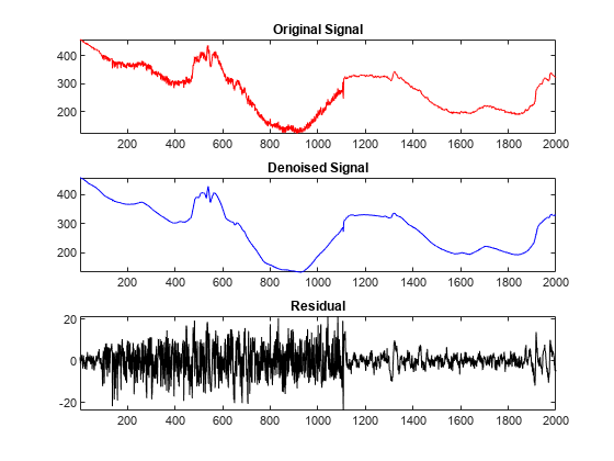
perf0,perfl2

perf0 = 
94.7860

perfl2 = 
99.9564

The denoised signal is very smooth. It seems quite good, but if we look at the residual after position 1100, we can see that the variance of the underlying noise is not constant. Some components of the signal have likely remained in the residual, such as, near the position 1300 and between positions 1900 and 2000.

Denoising Using the Interval Dependent Thresholds (IDT)

Now we will use an interval-dependent thresholding.

Perform a discrete wavelet analysis of the signal.

[coefs,longs] = wavedec(sig,level,wname);

Define the interval-dependent thresholds. Specify thresholds for three intervals:

I1 = [1 94] with a threshold of 5.9
I2 = [94 1110] with a threshold of 19.5
I3 = [1110 2000] with a threshold of 4.5

Define the interval-dependent thresholds.

denPAR = {[1 94 5.9 ; 94 1110 19.5 ; 1110 2000 4.5]};
thrParams = cell(1,level);
thrParams(:) = denPAR;

Show the wavelet coefficients of the signal and the interval-dependent threshold for each level of the discrete analysis.

% Replicate the coefficients
cfs_beg = wrepcoef(coefs,longs);

% Display the coefficients of the decomposition
figure
subplot(6,1,1)
plot(sig,'r')
axis tight
title('Original Signal and Detail Coefficients from 1 to 5')
ylabel('S','Rotation',0)
for k = 1:level
    subplot(6,1,k+1)
    plot(cfs_beg(k,:),'Color',[0.5 0.8 0.5])
    ylabel(['D' int2str(k)],'Rotation',0)
    axis tight 
    hold on
    maxi = max(abs(cfs_beg(k,:)));
    par = thrParams{k};
    plotPar = {'Color','m','LineStyle','-.'};
    for j = 1:size(par,1)-1
        plot([par(j,2),par(j,2)],[-maxi maxi],plotPar{:})
    end
    for j = 1:size(par,1)
        plot([par(j,1),par(j,2)],[par(j,3) par(j,3)],plotPar{:})
        plot([par(j,1),par(j,2)],-[par(j,3) par(j,3)],plotPar{:})            
    end
    ylim([-maxi*1.05 maxi*1.05])
    hold off
end
subplot(6,1,level+1)
xlabel('Time or Space')

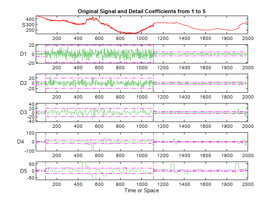
For each level k, the variable thrParams{k} contains the intervals and the corresponding thresholds for the denoising procedure.

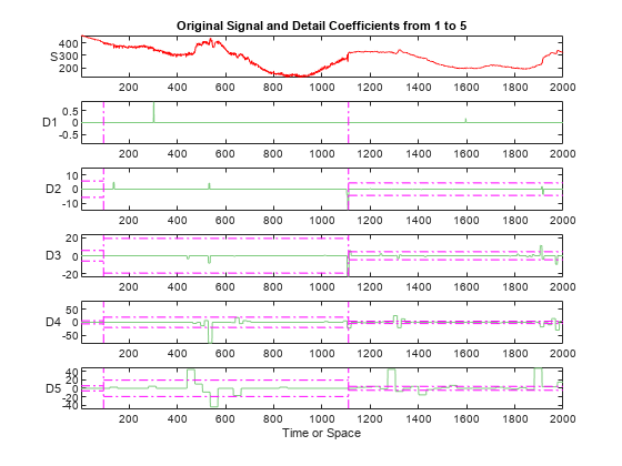
Threshold the wavelet coefficients level-by-level, and interval-by-interval, using the values contained in the thrParams variable.

Using the function wthresh, we threshold the wavelet coefficients values between the horizontal lines by replacing them with zeros, while other values are either reduced if sorh = 's' or remain unchanged if sorh = 'h'.

first = cumsum(longs)+1;
first = first(end-2:-1:1);
tmp   = longs(end-1:-1:2);
last  = first+tmp-1;
for k = 1:level
    thr_par = thrParams{k};
    if ~isempty(thr_par)
        cfs = coefs(first(k):last(k));
        nbCFS = longs(end-k);
        NB_int = size(thr_par,1);
        x = [thr_par(:,1) ; thr_par(NB_int,2)];
        alf = (nbCFS-1)/(x(end)-x(1));
        bet = 1 - alf*x(1);
        x = round(alf*x+bet);
        x(x<1) = 1;
        x(x>nbCFS) = nbCFS;
        thr = thr_par(:,3);
        for j = 1:NB_int
            if j == 1
                d_beg = 0; 
            else
                d_beg = 1;
            end
            j_beg = x(j)+ d_beg;
            j_end = x(j+1);
            j_ind = (j_beg:j_end);
            cfs(j_ind) = wthresh(cfs(j_ind),sorh,thr(j));
        end
        coefs(first(k):last(k)) = cfs;
    end
end

Show the thresholded wavelet coefficients of the signal.

% Replicate the coefficients.
cfs_beg = wrepcoef(coefs,longs);

% Display the decomposition coefficients.
figure
subplot(6,1,1)
plot(sig,'r')
axis tight
title('Original Signal and Detail Coefficients from 1 to 5')
ylabel('S','Rotation',0)
for k = 1:level
    subplot(6,1,k+1)
    plot(cfs_beg(k,:),'Color',[0.5 0.8 0.5])
    ylabel(['D' int2str(k)],'Rotation',0)
    axis tight
    hold on
    maxi = max(abs(cfs_beg(k,:)));
    par = thrParams{k};
    plotPar = {'Color','m','LineStyle','-.'};
    for j = 1:size(par,1)-1
        plot([par(j,2),par(j,2)],[-maxi maxi],plotPar{:})
    end
    for j = 1:size(par,1)
        plot([par(j,1),par(j,2)], [par(j,3) par(j,3)],plotPar{:})
        plot([par(j,1),par(j,2)],-[par(j,3) par(j,3)],plotPar{:})
    end
    ylim([-maxi*1.05 maxi*1.05])
    hold off
end
subplot(6,1,level+1)
xlabel('Time or Space')

Reconstruct the denoised signal.

sigden = waverec(coefs,longs,wname);
res = sig - sigden;

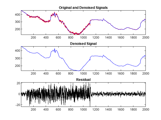
Display the original, denoised, and residual signals.

figure
subplot(3,1,1)
plot(sig,'r')
hold on 
plot(sigden,'b')
hold off
axis tight
title('Original and Denoised Signals')
subplot(3,1,2)
plot(sigden,'b')
axis tight
title('Denoised Signal')
subplot(3,1,3)
plot(res,'k')
axis tight
title('Residual')

Figure contains 3 axes objects. Axes object 1 with title Original and Denoised Signals contains 2 objects of type line. Axes object 2 with title Denoised Signal contains an object of type line. Axes object 3 with title Residual contains an object of type line.

Compare the three denoised versions of the signal.

figure
plot(sigden_1,'g')
hold on 
plot(sigden_2,'r')
plot(sigden,'k')
axis tight
hold off
legend('Denoised Min','Denoised Max','Denoised IDT','Location','North')

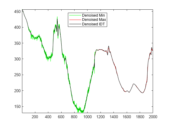
Figure contains an axes object. The axes object contains 3 objects of type line. These objects represent Denoised Min, Denoised Max, Denoised IDT.

Looking at the first half of the signals, it is clear that denoising using the minimum value of the threshold is not good. Now, we zoom on the end of the signal for more details.

xlim([1200 2000])
ylim([180 350])

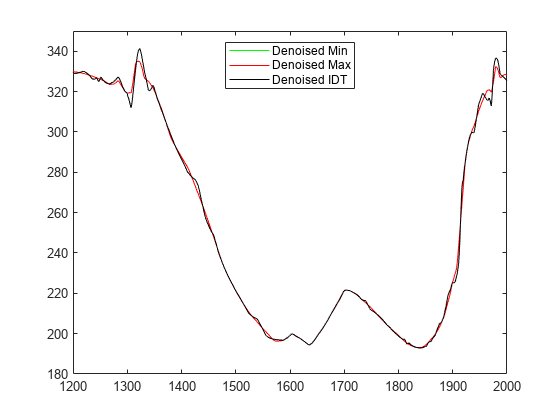
Figure contains an axes object. The axes object contains 3 objects of type line. These objects represent Denoised Min, Denoised Max, Denoised IDT.

We can see that when the maximum threshold value is used, the denoised signal is smoothed too much and information is lost.

The best result is given by using the threshold based on the interval- dependent thresholding method, as we will show now.

Automatic Computation of Interval-Dependent Thresholds

Instead of manually setting the intervals and the thresholds for each level, we can use the function utthrset_cmd to automatically compute the intervals and the thresholds for each interval. Then, we complete the procedure by applying the thresholds, reconstructing, and displaying the signal.

% Wavelet Analysis.
[coefs,longs] = wavedec(sig,level,wname);
siz = size(coefs);
thrParams = utthrset_cmd(coefs,longs);
first = cumsum(longs)+1;
first = first(end-2:-1:1);
tmp   = longs(end-1:-1:2);
last  = first+tmp-1;
for k = 1:level
    thr_par = thrParams{k};
    if ~isempty(thr_par)
        cfs = coefs(first(k):last(k));
        nbCFS = longs(end-k);
        NB_int = size(thr_par,1);
        x = [thr_par(:,1) ; thr_par(NB_int,2)];
        alf = (nbCFS-1)/(x(end)-x(1));
        bet = 1 - alf*x(1);
        x = round(alf*x+bet);
        x(x<1) = 1;
        x(x>nbCFS) = nbCFS;
        thr = thr_par(:,3);
        for j = 1:NB_int
            if j==1
                d_beg = 0;
            else
                d_beg = 1;
            end
            j_beg = x(j)+d_beg;
            j_end = x(j+1);
            j_ind = (j_beg:j_end);
            cfs(j_ind) = wthresh(cfs(j_ind),sorh,thr(j));
        end
        coefs(first(k):last(k)) = cfs;
    end
end
sigden = waverec(coefs,longs,wname);
figure
subplot(2,1,1)
plot(sig,'r')
axis tight
hold on
plot(sigden,'k')
title('Original and Denoised Signals')
subplot(2,1,2)
plot(sigden,'k')
axis tight
hold off
title('Denoised Signal')

Figure contains 2 axes objects. Axes object 1 with title Original and Denoised Signals contains 2 objects of type line. Axes object 2 with title Denoised Signal contains an object of type line.

Automatic Interval-Dependent Denoising

We can use the function cmddenoise to automatically compute the denoised signal and coefficients based on the interval-dependent denoising method. This method performs the whole process of denoising using only this one function, which includes all the steps described earlier in this example.

[sigden,~,thrParams] = cmddenoise(sig,wname,level);
thrParams{1}   % Denoising parameters for level 1.

ans = 2×3
10³ ×

    0.0010    1.1100    0.0176
    1.1100    2.0000    0.0045

The automatic procedure finds two intervals for denoising:

I1 = [1 1110] with a threshold of 17.6
I2 = [1110 2000] with a threshold of 4.5

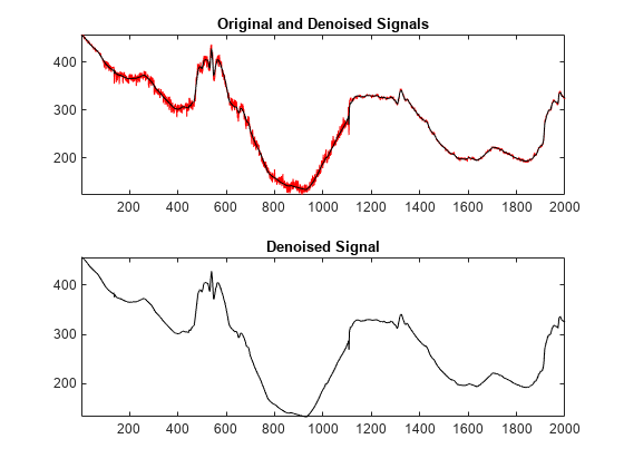
We can display the result of denoising and see that the result is fine.

figure
subplot(2,1,1)
plot(sig,'r')
axis tight
hold on
plot(sigden,'k')
title('Original and Denoised Signals')
hold off
subplot(2,1,2)
plot(sigden,'k')
axis tight
title('Denoised Signal')

Figure contains 2 axes objects. Axes object 1 with title Original and Denoised Signals contains 2 objects of type line. Axes object 2 with title Denoised Signal contains an object of type line.

Advanced Automatic Interval-Dependent Denoising

Now, we look at a more complete example of the automatic denoising.

Rather than using the default values for the input parameters, we can specify them when calling the function. Here, the type of threshold is chosen as 's' (soft) and the number of intervals is set at 3.

sig = nelec;                   % Signal to analyze.
wname  = 'sym4';               % Wavelet for analysis.
level  = 5;                    % Level for wavelet decomposition.
sorh   = 's';                  % Type of thresholding.
nb_Int = 3;                    % Number of intervals for thresholding.

[sigden,coefs,thrParams,int_DepThr_Cell,BestNbOfInt] = ...
            cmddenoise(sig,wname,level,sorh,nb_Int);

For the output parameters, the variable thrParams{1} gives the denoising parameters for levels from 1 to 5. For example, here are the denoising parameters for level 1.

thrParams{1}

ans = 3×3
10³ ×

    0.0010    0.0940    0.0059
    0.0940    1.1100    0.0195
    1.1100    2.0000    0.0045

We find the same values that were set earlier this example. They correspond to the choice we have made by fixing the number of intervals to three in the input parameter: nb_Int = 3.

The automatic procedure suggests 2 as the best number of intervals for denoising. This output value BestNbOfInt = 2 is the same as used in the previous step of this example.

BestNbOfInt

BestNbOfInt = 
2

The variable int_DepThr_Cell contains the interval locations and the threshold values for a number of intervals from 1 to 6.

cellfun(@size,int_DepThr_Cell,'UniformOutput',false)

ans=1×6 cell array
    {[1 3]}    {[2 3]}    {[3 3]}    {[4 3]}    {[5 3]}    {[6 3]}

Finally, we look at the values corresponding to the locations and thresholds for five intervals.

int_DepThr_Cell{5}

ans = 5×3
10³ ×

    0.0010    0.0940    0.0059
    0.0940    0.5420    0.0184
    0.5420    0.5640    0.0056
    0.5640    1.1100    0.0240
    1.1100    2.0000    0.0045

Summary

This example shows how to perform interval-dependent denoising.