Wavelet Denoising and Nonparametric Function Estimation
The Wavelet Toolbox™ provides a number of functions for the estimation of an unknown function (signal or image) in noise. You can use these functions to denoise signals and as a method for nonparametric function estimation.
The most general 1-D model for this is
s(n) = f(n) + σe(n)
where n= 0,1,2,...N-1. The e(n) are Gaussian random variables distributed as N(0,1). The variance of the σe(n) is σ2.
In practice, s(n) is often a discrete-time signal with equal time steps corrupted by additive noise and you are attempting to recover that signal.
More generally, you can view s(n) as an N-dimensional random vector
In this general context, the relationship between denoising and regression is clear.
You can replace the N-by-1 random vector by N-by-M random matrices to obtain the problem of recovering an image corrupted by additive noise.
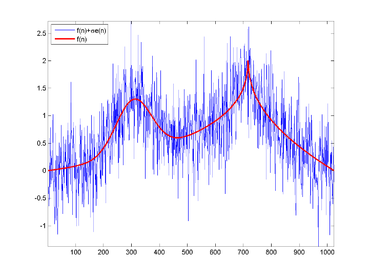
You can obtain a 1-D example of this model with the following code.
load cuspamax;
y = cuspamax+0.5*randn(size(cuspamax));
plot(y); hold on;
plot(cuspamax,'r','linewidth',2);
axis tight;
legend('f(n)+\sigma e(n)','f(n)', 'Location', 'NorthWest');
For a broad class of functions (signals, images) that possess certain smoothness properties, wavelet techniques are optimal or near optimal for function recovery.
Specifically, the method is efficient for families of functions f that have only a few nonzero wavelet coefficients. These functions have a sparse wavelet representation. For example, a smooth function almost everywhere, with only a few abrupt changes, has such a property.
The general wavelet–based method for denoising and nonparametric function estimation is to transform the data into the wavelet domain, threshold the wavelet coefficients, and invert the transform.
You can summarize these steps as:
Decompose
Choose a wavelet and a level N. Compute the wavelet decomposition of the signal s down to level N.
Threshold detail coefficients
For each level from 1 to N, threshold the detail coefficients.
Reconstruct
Compute wavelet reconstruction using the original approximation coefficients of level N and the modified detail coefficients of levels from 1 to N.
Denoising Methods
The Wavelet Toolbox supports a number of denoising methods. Four denoising methods are
implemented in the
thselect. Each method corresponds
to a tptr option in the command
thr = thselect(y,tptr)
which returns the threshold value.
Option | Denoising Method |
|---|---|
'rigrsure' | Selection using principle of Stein's Unbiased Risk Estimate (SURE) |
'sqtwolog' | Fixed form (universal) threshold equal to with N the length of the signal. |
'heursure' | Selection using a mixture of the first two options |
'minimaxi' |
Option
'rigrsure'uses for the soft threshold estimator a threshold selection rule based on Stein's Unbiased Estimate of Risk (quadratic loss function). You get an estimate of the risk for a particular threshold value t. Minimizing the risks in t gives a selection of the threshold value.Option
'sqtwolog'uses a fixed form threshold yielding minimax performance multiplied by a small factor proportional to log(length(s)).Option
'heursure'is a mixture of the two previous options. As a result, if the signal-to-noise ratio is very small, the SURE estimate is very noisy. So if such a situation is detected, the fixed form threshold is used.Option
'minimaxi'uses a fixed threshold chosen to yield minimax performance for mean square error against an ideal procedure. The minimax principle is used in statistics to design estimators. Since the denoised signal can be assimilated to the estimator of the unknown regression function, the minimax estimator is the option that realizes the minimum, over a given set of functions, of the maximum mean square error.
The following example shows the denoising methods for a 1000-by-1 N(0,1) vector. The signal here is
with f(n) = 0.
rng default;
sig = randn(1e3,1);
thr_rigrsure = thselect(sig,'rigrsure')
thr_univthresh = thselect(sig,'sqtwolog')
thr_heursure = thselect(sig,'heursure')
thr_minimaxi = thselect(sig,'minimaxi')
histogram(sig);
h = findobj(gca,'Type','patch');
set(h,'FaceColor',[0.7 0.7 0.7],'EdgeColor','w');
hold on;
plot([thr_rigrsure thr_rigrsure], [0 300],'linewidth',2);
plot([thr_univthresh thr_univthresh], [0 300],'r','linewidth',2);
plot([thr_minimaxi thr_minimaxi], [0 300],'k','linewidth',2);
plot([-thr_rigrsure -thr_rigrsure], [0 300],'linewidth',2);
plot([-thr_univthresh -thr_univthresh], [0 300],'r','linewidth',2);
plot([-thr_minimaxi -thr_minimaxi], [0 300],'k','linewidth',2);
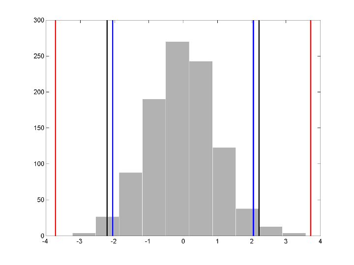
For Stein's Unbiased Risk Estimate (SURE) and minimax thresholds, approximately 3% of coefficients are retained. In the case of the universal threshold, all values are rejected.
We know that the detail coefficients vector is the superposition of the coefficients of f and the coefficients of e, and that the decomposition of e leads to detail coefficients, which are standard Gaussian white noises.
After you use thselect to determine a
threshold, you can threshold each level of a wavelet decomposition. This second step
can be done using wthcoef, directly handling the wavelet
decomposition structure of the original signal s.
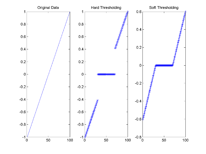
Soft or Hard Thresholding
Hard and soft thresholding are examples of shrinkage rules. After you have determined your threshold, you have to decide how to apply that threshold to your data.
The simplest scheme is hard thresholding. Let T denote the threshold and x your data. The hard thresholding is
The soft thresholding is
You can apply your threshold using the hard or soft rule with wthresh.
y = linspace(-1,1,100);
thr = 0.4;
ythard = wthresh(y,'h',thr);
ytsoft = wthresh(y,'s',thr);
subplot(131);
plot(y); title('Original Data');
subplot(132);
plot(ythard,'*'); title('Hard Thresholding');
subplot(133);
plot(ytsoft,'*'); title('Soft Thresholding');
Dealing with Unscaled Noise and Nonwhite Noise
Usually in practice the basic model cannot be used directly. We examine here the
options available to deal with model deviations in the main denoising function
wdenoise.
The simplest use of wdenoise
is
sd = wdenoise(s)
sd of the original signal s obtained
by using default settings for parameters including wavelet, denoising method, and
soft or hard thresholding. Any of the default settings can be
changed:sd = wdenoise(s,n,'DenoisingMethod',tptr,'Wavelet',wav,...
'ThresholdRule',sorh,'NoiseEstimate',scal)sd of the original signal
s obtained using the tptr denoising
method. Other parameters needed are sorh,
scal, and wname. The parameter
sorh specifies the thresholding of details coefficients of
the decomposition at level n of s by the
wavelet called wav. The remaining parameter
scal is to be specified. It corresponds to the method of
estimating variance of noise in the data.
Option | Noise Estimate Method |
|---|---|
'LevelIndependent' |
|
'LevelDependent' |
|
For a more general procedure, the wdencmp function
performs wavelet coefficients thresholding for both denoising and
compression purposes, while directly handling 1-D and 2-D data. It
allows you to define your own thresholding strategy selecting in
xd = wdencmp(opt,x,wav,n,thr,sorh,keepapp);
where
opt = 'gbl'andthris a positive real number for uniform threshold.opt = 'lvd'andthris a vector for level dependent threshold.keepapp = 1to keep approximation coefficients, as previously andkeepapp = 0to allow approximation coefficients thresholding.xis the signal to be denoised andwav,n,sorhare the same as above.
Wavelet Denoising in Action
We begin the examples of 1-D denoising methods with the first example credited to Donoho and Johnstone.
Blocks Signal Thresholding
First set a signal-to-noise ratio (SNR) and set a random seed.
sqrt_snr = 4;
init = 2055615866;
Generate an original signal xref and a noisy version x by adding standard Gaussian white noise. Plot both signals.
[xref,x] = wnoise(1,11,sqrt_snr,init);
subplot(2,1,1)
plot(xref)
axis tight
title('Original Signal')
subplot(2,1,2)
plot(x)
axis tight
title('Noisy Signal')

Denoise the noisy signal using soft heuristic SURE thresholding on detail coefficients obtained from the wavelet decomposition of x using the sym8 wavelet. Use the default settings of wdenoise for the remaining parameters. Compare with the original signal.
xd = wdenoise(x,'Wavelet','sym8','DenoisingMethod','SURE','ThresholdRule','Soft');
figure
subplot(2,1,1)
plot(xref)
axis tight
title('Original Signal')
subplot(2,1,2)
plot(xd)
axis tight
title('Denoised Signal')
Since only a small number of large coefficients characterize the original signal, the method performs very well.
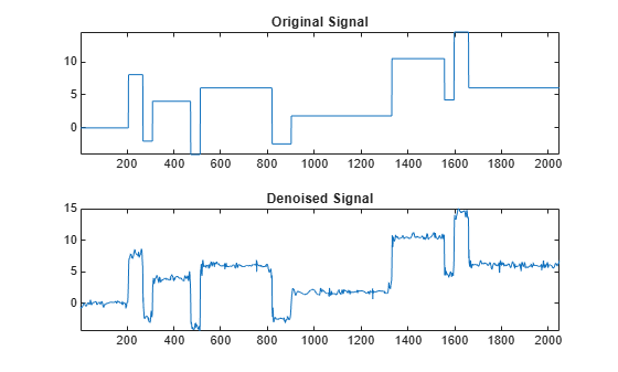
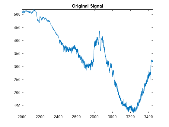
Electrical Signal Denoising
When you suspect a non-white noise, thresholds must be rescaled by a level-dependent estimation of the level noise. As a second example, let us try the method on the highly perturbed part of an electrical signal.
First load the electrical signal and select a segment from it. Plot the segment.
load leleccum
indx = 2000:3450;
x = leleccum(indx);
figure
plot(indx,x)
axis tight
title('Original Signal')
Denoise the signal using the db3 wavelet and a three-level wavelet decomposition and soft fixed form thresholding. To deal with the non-white noise, use level-dependent noise size estimation. Compare with the original signal.
xd = wdenoise(x,3,'Wavelet','db3',...
    'DenoisingMethod','UniversalThreshold',...
    'ThresholdRule','Soft',...
    'NoiseEstimate','LevelDependent');
figure
subplot(2,1,1)
plot(indx,x)
axis tight
title('Original Signal')
subplot(2,1,2)
plot(indx,xd)
axis tight
title('Denoised Signal')
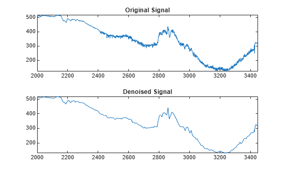
The result is quite good in spite of the time heterogeneity of the nature of the noise after and before the beginning of the sensor failure around time 2410.
Extension to Image Denoising
The denoising method described for the 1-D case applies also to images and applies well to geometrical images. A direct translation of the 1-D model is
where is a white Gaussian noise with unit variance.
The 2-D denoising procedure has the same three steps and uses 2-D wavelet tools instead of 1-D tools. For the threshold selection, prod(size(s)) is used instead of length(s) if the fixed form threshold is used.
Note that except for the "automatic" 1-D denoising case, 2-D denoising and compression are performed using wdencmp. To illustrate 2-D denoising, load an image and create a noisy version of it. For purposes of reproducibility, set the random seed.
init = 2055615866;
rng(init);
load woman
img = X;
imgNoisy = img + 15*randn(size(img));
Use ddencmp to find the denoising values. In this case, fixed form threshold is used with estimation of level noise, thresholding is soft and the approximation coefficients are kept.
[thr,sorh,keepapp] = ddencmp('den','wv',imgNoisy);
thr
thr =
107.9838
thr is equal to estimated_sigma*sqrt(log(prod(size(img)))).
Denoise the noisy image using the global threshold option. Display the results.
imgDenoised = wdencmp('gbl',imgNoisy,'sym4',2,thr,sorh,keepapp);
figure
colormap(pink(255))
sm = size(map,1);
subplot(2,2,1)
image(wcodemat(img,sm))
title('Original Image')
subplot(2,2,2)
image(wcodemat(imgNoisy,sm))
title('Noisy Image')
subplot(2,2,3)
image(wcodemat(imgDenoised,sm))
title('Denoised Image')
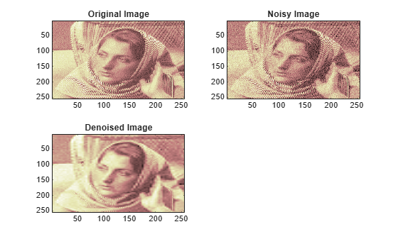
The denoised image compares well with the original image.
1-D Wavelet Variance Adaptive Thresholding
The idea is to define level by level time-dependent thresholds, and then increase the capability of the denoising strategies to handle nonstationary variance noise models.
More precisely, the model assumes (as previously) that the observation is equal to the interesting signal superimposed on noise
But the noise variance can vary with time. There are several different variance values on several time intervals. The values as well as the intervals are unknown.
Let us focus on the problem of estimating the change points or equivalently the intervals. The algorithm used is based on an original work of Marc Lavielle about detection of change points using dynamic programming (see [Lav99] in References).
Let us generate a signal from a fixed-design regression model with two noise variance change points located at positions 200 and 600. For purposes of reproducibility, set the random seed.
init = 2055615866;
rng(init);

x = wnoise(1,10);
bb = randn(1,length(x));
cp1 = 200;
cp2 = 600;
x = x+[bb(1:cp1),bb(cp1+1:cp2)/4,bb(cp2+1:end)];
plot(x)
title('Noisy Signal')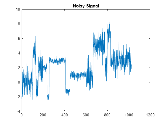
The aim of this example is to recover the two change points from the signal x.
Step 1. Recover a noisy signal by suppressing an approximation. First perform a single-level wavelet decomposition using the db3 wavelet. Then reconstruct the detail at level 1.
wname = 'db3';
lev = 1;
[c,l] = wavedec(x,lev,wname);
det = wrcoef('d',c,l,wname,1);
figure
plot(det)
title('Level 1 Detail')
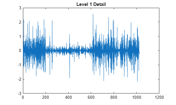
The reconstructed detail at level 1 recovered at this stage is almost signal free. It captures the main features of the noise from a change points detection viewpoint if the interesting part of the signal has a sparse wavelet representation. To remove almost all the signal, we replace the biggest values by the mean.
Step 2. To remove almost all the signal, replace 2% of biggest values by the mean.
x = sort(abs(det));
v2p100 = x(fix(length(x)*0.98));
ind = find(abs(det)>v2p100);
det(ind) = mean(det);
Step 3. Use the wvarchg function to estimate the change points with the following parameters:
The minimum delay between two change points is d = 10.
The maximum number of change points is 5.
[cp_est,kopt,t_est] = wvarchg(det,5)
cp_est = 1×2

   259   611
kopt =
2
t_est = 6×6

        1024           0           0           0           0           0
         612        1024           0           0           0           0
         259         611        1024           0           0           0
         198         259         611        1024           0           0
         198         235         259         611        1024           0
         198         235         260         346         611        1024
Two change points and three intervals are proposed. Since the three interval variances for the noise are very different the optimization program detects easily the correct structure. The estimated change points are close to the true change points: 200 and 600.
Step 4. (Optional) Replace the estimated change points.
For 2 i 6, t_est(i,1:i-1) contains the i-1 instants of the variance change points, and since kopt is the proposed number of change points, then
cp_est = t_est(kopt+1,1:kopt);
You can replace the estimated change points by computing:
for k=1:5
    cp_New = t_est(k+1,1:k)
end
cp_New =
612
cp_New = 1×2

   259   611
cp_New = 1×3

   198   259   611
cp_New = 1×4

   198   235   259   611
cp_New = 1×5

   198   235   260   346   611
Wavelet Denoising Analysis Measurements
The following measurements and settings are useful for analyzing wavelet signals and images:
M S E — Mean square error (MSE) is the squared norm of the difference between the data and the signal or image approximation divided by the number of elements.
Max Error — Maximum absolute squared deviation in the signal or image approximation.
L2-Norm Ratio — Ratio of the squared L2-norm of the signal or image approximation to the input signal or image. For images, the image is reshaped as a column vector before taking the L2-norm
P S N R — Peak signal-to-noise ratio (PSNR) in decibels. PSNR is meaningful only for data encoded in terms of bits per sample or bits per pixel.
B P P — Bits per pixel ratio (BPP), which is the compression ratio (Comp. Ratio) multiplied by 8, assuming one byte per pixel (8 bits).
Comp Ratio — Compression ratio, which is the number of elements in the compressed image divided by the number of elements in the original image expressed as a percentage.