1-D Multisignal Analysis

This section takes you through the features of 1-D multisignal wavelet analysis, compression and denoising using the Wavelet Toolbox™ software. The rationale for each topic is the same as in the 1-D single signal case.

The toolbox provides the following functions for multisignal analysis.

Analysis-Decomposition and Synthesis-Reconstruction Functions

Function Name	Purpose
`mdwtdec`	Multisignal wavelet decomposition
`mdwtrec`	Multisignal wavelet reconstruction and extraction of approximation and detail coefficients

Decomposition Structure Utilities

Function Name	Purpose
`chgwdeccfs`	Change multisignal 1-D decomposition coefficients
`wdecenergy`	Multisignal 1-D decomposition energy repartition

Compression and Denoising Functions

Function Name	Purpose
`mswcmp`	Multisignal 1-D compression using wavelets
`mswcmpscr`	Multisignal 1-D wavelet compression scores
`mswcmptp`	Multisignal 1-D compression thresholds and performance
`mswden`	Multisignal 1-D denoising using wavelets
`mswthresh`	Perform multisignal 1-D thresholding

1-D Multisignal Analysis

Load a file, from the MATLAB^® prompt, by typing
```
load thinker
```
The file thinker.mat contains a single variable X. Use whos to show information about X.
```
whos
```
Name Size Bytes Class
X 192x96 147456 double array

Name	Size	Bytes	Class
`X`	`192x96`	`147456`	`double array`

Plot some signals.

figure;
plot(X(1:5,:)','r');   hold on 
plot(X(21:25,:)','b'); plot(X(31:35,:)','g')
set(gca,'Xlim',[1,96]) 
grid

Perform a wavelet decomposition of signals at level 2 of row signals using the db2 wavelet.

dec = mdwtdec('r',X,2,'db2')

This generates the decomposition structure dec:

dec =
         dirDec: 'r'
          level: 2
          wname: 'db2'
     dwtFilters: [1x1 struct]
        dwtEXTM: 'sym'
       dwtShift: 0
       dataSize: [192 96]
             ca: [192x26 double]
             cd: {[192x49 double]  [192x26 double]}

Change wavelet coefficients.
For each signal change the wavelet coefficients by setting all the coefficients of the detail of level 1 to zero.
```
decBIS = chgwdeccfs(dec,'cd',0,1);
```
This generates a new decomposition structure decBIS.

Perform a wavelet reconstruction of signals and plot some of the new signals.

Xbis = mdwtrec(decBIS); 
figure;  
plot(Xbis(1:5,:)','r');   hold on 
plot(Xbis(21:25,:)','b');
plot(Xbis(31:35,:)','g') 
grid; set(gca,'Xlim',[1,96])

Compare old and new signals by plotting them together.

figure; idxSIG = [1 31]; 
plot(X(idxSIG,:)','r','linewidth',2);   hold on 
plot(Xbis(idxSIG,:)','b','linewidth',2);
grid; set(gca,'Xlim',[1,96])

Set the wavelet coefficients at level 1 and 2 for signals 31 to 35 to the value zero, perform a wavelet reconstruction of signal 31, and compare some of the old and new signals.

decTER = chgwdeccfs(dec,'cd',0,1:2,31:35); 
Y = mdwtrec(decTER,'a',0,31);
figure; 
plot(X([1 31],:)','r','linewidth',2);   hold on 
plot([Xbis(1,:)
; Y]','b','linewidth',2); 
grid; set(gca,'Xlim',[1,96])

Compute the energy of signals and the percentage of energy for wavelet components.

[E,PEC,PECFS] = wdecenergy(dec);

Energy of signals 1 and 31:

Ener_1_31 = E([1 31])
Ener_1_31 = 

  1.0e+006 * 
    3.7534 
    2.2411

Compute the percentage of energy for wavelet components of signals 1 and 31.
```
PEC_1_31 = PEC([1 31],:)  

PEC_1_31 = 
   99.7760    0.1718    0.0522 
   99.3850    0.2926    0.3225
```
The first column shows the percentage of energy for approximations at level 2. Columns 2 and 3 show the percentage of energy for details at level 2 and 1, respectively.
Display the percentage of energy for wavelet coefficients of signals 1 and 31. As we can see in the dec structure, there are 26 coefficients for the approximation and the detail at level 2, and 49 coefficients for the detail at level 1.
```
PECFS_1 = PECFS(1,:); PECFS_31 = PECFS(31,:); 
figure; 
plot(PECFS_1,'r','linewidth',2); hold on 
plot(PECFS_31,'b','linewidth',2); 
grid; set(gca,'Xlim',[1,size(PECFS,2)])
```

Compress the signals to obtain a percentage of zeros near 95% for the wavelet coefficients.

[XC,decCMP,THRESH] = mswcmp('cmp',dec,'N0_perf',95); 
[Ecmp,PECcmp,PECFScmp] = wdecenergy(decCMP);

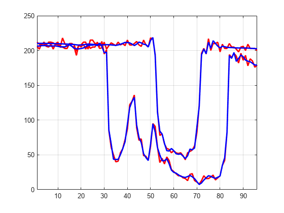
Plot the original signals 1 and 31, and the corresponding compressed signals.

figure;
plot(X([1 31],:)','r','linewidth',2);   hold on 
plot(XC([1 31],:)','b','linewidth',2);
grid; set(gca,'Xlim',[1,96])

Compute thresholds, percentage of energy preserved and percentage of zeros associated with the L2_perf method preserving at least 95% of energy.

[THR_VAL,L2_Perf,N0_Perf] = mswcmptp(dec,'L2_perf',95); 
idxSIG = [1,31];  

Thr   = THR_VAL(idxSIG)
Thr = 
  256.1914 
  158.6085 

L2per = L2_Perf(idxSIG) 
L2per =  
  96.5488
  94.7197

N0per = N0_Perf(idxSIG) 
N0per = 
  79.2079  
  86.1386

Compress the signals to obtain a percentage of zeros near 60% for the wavelet coefficients.

[XC,decCMP,THRESH] = mswcmp('cmp',dec,'N0_perf',60);

XC signals are the compressed versions of the original signals in the row direction.

Compress the XC signals in the column direction

XX = mswcmp('cmpsig','c',XC,'db2',2,'N0_perf',60);

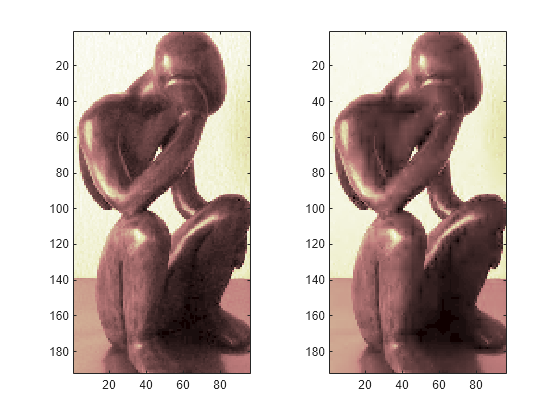
Plot original signals X and the compressed signals XX as images.

figure;
subplot(1,2,1); image(X) 
subplot(1,2,2); image(XX) 
colormap(pink(222))

Denoise the signals using the universal threshold:

[XD,decDEN,THRESH] = mswden('den',dec,'sqtwolog','sln'); figure; 
plot(X([1 31],:)','r','linewidth',2); hold on 
plot(XD([1 31],:)','b','linewidth',2); 
grid; set(gca,'Xlim',[1,96])

XD signals are the denoised versions of the original signals in the row direction.

Denoise the XD signals in column direction

XX = mswden('densig','c',XD,'db2',2,'sqtwolog','sln');

Plot original signals X and the denoised signals XX as images.

figure;
subplot(1,2,1); image(X) 
subplot(1,2,2); image(XX) 
colormap(pink(222))

References

[1] Denoeud, L., Garreta, H., and A. Guénoche. "Comparison of Distance Indices Between Partitions." In International Symposium on Applied Stochastic Models and Data Analysis, 432–440. Brest, France: École Nationale des Télécommunications de Bretagne, 2005.