1-D Stationary Wavelet Transform

This topic takes you through the features of 1-D discrete stationary wavelet analysis using the Wavelet Toolbox™ software. For more information see Nondecimated Discrete Stationary Wavelet Transforms (SWTs) in the Wavelet Toolbox User's Guide.

The toolbox provides these functions for 1-D discrete stationary wavelet analysis. For more information on the functions, see the reference pages.

Analysis-Decomposition Functions

Function Name	Purpose
`swt`	Decomposition

Synthesis-Reconstruction Functions

Function Name	Purpose
`iswt`	Reconstruction

The stationary wavelet decomposition structure is more tractable than the wavelet one. So the utilities, useful for the wavelet case, are not necessary for the stationary wavelet transform (SWT).

In this section, you'll learn to

Load a signal
Perform a stationary wavelet decomposition of a signal
Construct approximations and details from the coefficients
Display the approximation and detail at level 1
Regenerate a signal by using inverse stationary wavelet transform
Perform a multilevel stationary wavelet decomposition of a signal
Reconstruct the level 3 approximation
Reconstruct the level 1, 2, and 3 details
Reconstruct the level 1 and 2 approximations
Display the results of a decomposition
Reconstruct the original signal from the level 3 decomposition
Remove noise from a signal

1-D Analysis

This example involves a noisy Doppler test signal.

Load a signal.
From the MATLAB^® prompt, type
```
load noisdopp
```
Set the variables. Type
```
s = noisdopp; 
```
For the SWT, if a decomposition at level k is needed, 2^k must divide evenly into the length of the signal. If your original signal does not have the correct length, you can use the wextend function to extend it.
Perform a single-level Stationary Wavelet Decomposition.
Perform a single-level decomposition of the signal using the db1 wavelet. Type
```
[swa,swd] = swt(s,1,'db1');
```
This generates the coefficients of the level 1 approximation (swa) and detail (swd). Both are of the same length as the signal. Type
```
whos
```
Name Size Bytes Class
noisdopp 1x1024 8192 double array
s 1x1024 8192 double array
swa 1x1024 8192 double array
swd 1x1024 8192 double array
Display the coefficients of approximation and detail.
To display the coefficients of approximation and detail at level 1, type
```
subplot(1,2,1), plot(swa); title('Approximation cfs') 
subplot(1,2,2), plot(swd); title('Detail cfs')
```
Regenerate the signal by Inverse Stationary Wavelet Transform.
To find the inverse transform, type
```
A0 = iswt(swa,swd,'db1'); 
```
To check the perfect reconstruction, type
```
err = norm(s-A0)
err = 
 2.1450e-14
```
Construct and display approximation and detail from the coefficients.
To construct the level 1 approximation and detail (A1 and D1) from the coefficients swa and swd, type
```
nulcfs = zeros(size(swa));
A1 = iswt(swa,nulcfs,'db1');  
D1 = iswt(nulcfs,swd,'db1');
```
To display the approximation and detail at level 1, type
```
subplot(1,2,1), plot(A1); title('Approximation A1'); 
subplot(1,2,2), plot(D1); title('Detail D1');
```
Perform a multilevel Stationary Wavelet Decomposition.
To perform a decomposition at level 3 of the signal (again using the db1 wavelet), type
```
[swa,swd] = swt(s,3,'db1');
```
This generates the coefficients of the approximations at levels 1, 2, and 3 (swa) and the coefficients of the details (swd). Observe that the rows of swa and swd are the same length as the signal length. Type
```
clear A0 A1 D1 err nulcfs 
whos
```
Name Size Bytes Class
noisdopp 1x1024 8192 double array
s 1x1024 8192 double array
swa 3x1024 24576 double array
swd 3x1024 24576 double array

Name	Size	Bytes	Class
`noisdopp`	`1x1024`	`8192`	`double array`
`s`	`1x1024`	`8192`	`double array`
`swa`	`1x1024`	`8192`	`double array`
`swd`	`1x1024`	`8192`	`double array`

Name	Size	Bytes	Class
`noisdopp`	`1x1024`	`8192`	`double array`
`s`	`1x1024`	`8192`	`double array`
`swa`	`3x1024`	`24576`	`double array`
`swd`	`3x1024`	`24576`	`double array`

Display the coefficients of approximations and details.

To display the coefficients of approximations and details, type

kp = 0; 
for i = 1:3
    subplot(3,2,kp+1), plot(swa(i,:));
    title(['Approx. cfs level ',num2str(i)])
    subplot(3,2,kp+2), plot(swd(i,:));  
    title(['Detail cfs level ',num2str(i)])
    kp = kp + 2; 
end

Reconstruct approximation at Level 3 From coefficients.
To reconstruct the approximation at level 3, type
```
mzero = zeros(size(swd)); 
A = mzero; 
A(3,:) = iswt(swa,mzero,'db1');
```

Reconstruct details from coefficients.

To reconstruct the details at levels 1, 2 and 3, type

D = mzero; 
for i = 1:3
    swcfs = mzero;
    swcfs(i,:) = swd(i,:);
    D(i,:) = iswt(mzero,swcfs,'db1');
end

Reconstruct and display approximations at Levels 1 and 2 from approximation at Level 3 and details at Levels 2 and 3.

To reconstruct the approximations at levels 2 and 3, type

A(2,:) = A(3,:) + D(3,:); 
A(1,:) = A(2,:) + D(2,:);

To display the approximations and details at levels 1, 2 and 3, type

kp = 0; 
for i = 1:3
    subplot(3,2,kp+1), plot(A(i,:));
    title(['Approx. level ',num2str(i)])
    subplot(3,2,kp+2), plot(D(i,:));
    title(['Detail level ',num2str(i)])
    kp = kp + 2;
end

Remove noise by thresholding.
To denoise the signal, use the ddencmp command to calculate a default global threshold. Use the wthresh command to perform the actual thresholding of the detail coefficients, and then use the iswt command to obtain the denoised signal.
Note
All methods for choosing thresholds in the 1-D Discrete Wavelet Transform case are also valid for the 1-D Stationary Wavelet Transform, which are also those used by the Wavelet Analysis app. This is also true for the 2-D transforms.

[thr,sorh] = ddencmp('den','wv',s); 
dswd = wthresh(swd,sorh,thr); 
clean = iswt(swa,dswd,'db1');

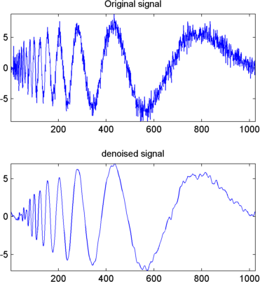
To display both the original and denoised signals, type

subplot(2,1,1), plot(s); 
title('Original signal') 
subplot(2,1,2), plot(clean); 
title('denoised signal')

The obtained signal remains a little bit noisy. The result can be improved by considering the decomposition of s at level 5 instead of level 3, and repeating steps 14 and 15. To improve the previous denoising, type

[swa,swd] = swt(s,5,'db1'); 
[thr,sorh] = ddencmp('den','wv',s); 
dswd = wthresh(swd,sorh,thr);
clean = iswt(swa,dswd,'db1'); 
subplot(2,1,1), plot(s); title('Original signal') 
subplot(2,1,2), plot(clean); title('denoised signal')

A second syntax can be used for the swt and iswt functions, giving the same results:

lev = 5; swc = swt(s,lev,'db1'); 
swcden = swc; 
swcden(1:end-1,:) = wthresh(swcden(1:end-1,:),sorh,thr);
clean = iswt(swcden,'db1');

You can obtain the same plot by using the same plot commands as in step 16 above.