Object Tracking Using 2-D FFT
This example shows how to implement an object tracking algorithm on FPGA. The model in this example supports a high frame rate of 1080p@120 fps.
High speed object tracking is essential for a number of computer vision tasks and includes applications ranging across automotive, aerospace and defense sectors. The main principle behind this tracking technique is adaptive template matching where the tracker detects the best match of a template within an input image region at each frame.
Download Input File
This example uses the quadrocopter.avi file from the Linkoping Thermal InfraRed (LTIR) data set [ 2 ] as input to the model. The file is approximately 3 MB in size. Download the file from the MathWorks website and unzip the downloaded file.
LTIRZipFile = matlab.internal.examples.downloadSupportFile('visionhdl','LTIR_dataset.zip');
[outputFolder,~,~] = fileparts(LTIRZipFile);
unzip(LTIRZipFile,outputFolder);
quadrocopterVideoFile = fullfile(outputFolder,'LTIR_dataset');
addpath(quadrocopterVideoFile);
Overview
The example model provides two subsystems, a behavioral design using the Computer Vision Toolbox™ and an HDL design using the Vision HDL Toolbox™ that supports HDL code generation. The ObjectTrackerHDL subsystem is the hardware part of the design and takes a pixel stream as input. The ROI Selector block dynamically selects an active region of the pixel stream that corresponds to a square search template. The model correlates the template with an initialized adaptive filter. The maximum point of correlation determines the new template location, which the model uses to shift the template in the next frame.
The ObjectTrackerHDL subsystem provides two configuration mask parameters:
ObjectCenter — The x- and y-coordinate pair that indicates the center of the object or the template.
templateSize — Size of the square template. The allowable sizes range from 16 to 256 in powers of 2.
modelname = 'ObjectTrackerHDL';
open_system(modelname);
set_param(modelname,'SampleTimeColors','on');
set_param(modelname,'SimulationCommand','Update');
set_param(modelname,'Open','on');
set(allchild(0),'Visible','off');
![]()
Object Tracker HDL Subsystem
The input to the design is a grayscale or thermal uint8 image. The input image can be of custom size. Thermal image tracking can involve additional challenges with fast motion and illumination variation. Therefore, a higher frame rate is usually desirable for most infrared (IR) applications.
The ObjectTrackerHDL design consists of the Preprocess, Tracking, and Overlay subsystems. The preprocess logic selects the template and does mean subtraction, variance normalization, and windowing to emphasize the target better. The tracking subsystem tracks the template across the frames. The overlay subsystem consists of the VideoOverlay subsystem. It accepts a pixel streaming input and takes the position of the template and overlays it onto the frame for viewing. It provides five color options and configurable opacity for better visualization.
open_system([modelname '/ObjectTrackerHDL'],'force');
![]()
Tracking Algorithm
The tracking algorithm uses a Minimum Output Sum of Squared Error[1] (MOSSE) filter for correlation. This type of filter tries to minimize the sum of squared error between the actual and desired correlation. The initial setup for tracking is a simple training procedure that happens at the initialization of the model. The InitFcn callback provides this setup. During setup, the model pretrains the filter using random affine transformations on the first frame template. The training output is a 2-D Gaussian centered on the training input. To suit your application better, you can update these variables in the InitFcn:
eta (
 ) — The learning rate or the weight given to the coefficients of the previous frame.
sigma — The gaussian variance or the sharpness of the target object.
trainCount — The number of training images used.
After the training procedure, the initial coefficients of the filter are available and loaded as constants in the model. This adaptive algorithm updates the filter coefficients after each frame. Let ![]() be the desired correlation output, then the algorithm tries to derive a filter
be the desired correlation output, then the algorithm tries to derive a filter ![]() , such that its correlation with the template
, such that its correlation with the template ![]() satisfies the following optimization equation.
satisfies the following optimization equation.
![]()
This equation can be solved as follows:
![]()
![]()
![]()
As the filter adapts to follow the object, the learning rate represents the effect of previous frames. The algorithm is iterative, so it correlates the given template is correlated with the filter and uses the maximum of correlation to guide the selection of the new template.
Track Subsystem
After preprocessing the pixel stream, the Track subsystem performs 2-D correlation between the initial template and the filter. First, the subsystem converts the template into the frequency domain using 2-D FFT. Because the data is now in the frequency domain, the subsystem efficiently implements correlation as element-wise multiplication. The MaxCorrelation subsystem finds the column and row in the template where the maximum value occurs. It streams in pixels and compares them to find the maximum value and the HV Counter block determines the location of this maximum value. If more than one maximum value exists, the subsystem finds the mean of the solutions. If the pixel value is already equal to the maximum value, the subsystem updates the location as the mean location corresponding to both values. The model repeats this process until it finds a new maximum value or it exhausts the number of pixels in the frame. The ROIUpdate subsystem updates the previous ROI by using the maximum point in correlation and shifting its center to the new maximum point to yield the current ROI.
open_system([modelname '/ObjectTrackerHDL/Track'],'force');
![]()
2-D Correlation Subsystem
The model performs 2-D correlation in the frequency domain. The 2-DCorrelation subsystem has two templates in process at each frame, i.e., previous and current ROI templates. The subsystem represents both templates at the frequency scale using 2-D FFT and uses the current template to update coefficients of the filter. The CoefficientsUpdate1 subsystem contains RAM blocks to store the coefficients, which it updates for use in the next frame. The subsystem stores the coefficients of the filter in the frequency domain. This format enables the design to use element-wise multiplication to calculate the correlation. The subsystem aligns the two pixel streams before multiplication and controls the alignment by comparing the previous and current ROI values. Finally, the subsystem converts the result back to time domain using an IFFT.
open_system([modelname '/ObjectTrackerHDL/Track/2-DCorrelation'],'force');
![]()
2-D FFT Subsystem
The subsystem calculates the 2-D FFT by performing a 1-D FFT across the rows of the template, storing the result, and performing a 1-D FFT across its columns. For more details, see FFT (DSP HDL Toolbox)(1-D). The CornerTurnMemory subsystem stores the result using ping-pong buffering, which enables high-speed read and write.
open_system([modelname '/ObjectTrackerHDL/Track/2-DCorrelation/Prev2-DFFT'],'force');
![]()
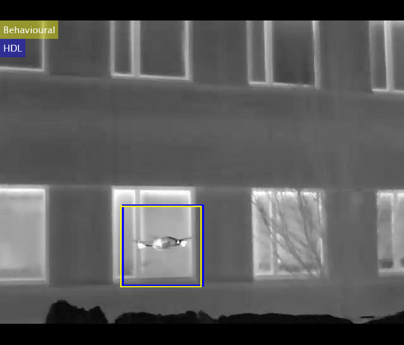
Simulation and Output
At the end of each frame, the model updates the video display for the behavioral and HDL designs. Although the two outputs closely follow each other, a slight deviation in one result can compound over a few frames. Both systems independently track the quadrocopter through the video. The quadrocopter sequence contains 480p uint8 images and the template size is set to 128 pixels.
Implementation Results
To generate HDL code from this example model, you must have the HDL Coder™ product. To generate HDL code, use this command.
makehdl('ObjectTrackerHDL/ObjectTrackerHDL')
The generated code was synthesized for an AMD® ZCU106 SoC device. The design meets a 285 MHz timing constraint for a template size of 128 pixels. The table shows the hardware resources used by the design.
T = table(...
    categorical({'DSP48';'Register';'LUT';'BRAM';'URAM'}), ...
    categorical({'260 (15.05%)';'65311 (14.17%)';'45414 (19.71%)';'95 (30.44%)';'36 (37.5%)'}), ...
    'VariableNames',{'Resource','Usage'})
T =

  5×2 table

    Resource        Usage
    ________    ______________

    DSP48       260 (15.05%)
    Register    65311 (14.17%)
    LUT         45414 (19.71%)
    BRAM        95 (30.44%)
    URAM        36 (37.5%)
References
[1] D. S. Bolme, J. R. Beveridge, B. A. Draper and Y. M. Lui, "Visual object tracking using adaptive correlation filters," 2010 IEEE Computer Society Conference on Computer Vision and Pattern Recognition, 2010, pp. 2544–2550, doi: 10.1109/CVPR.2010.5539960.
[2] A. Berg, J. Ahlberg and M. Felsberg, "A Thermal Object Tracking Benchmark," 2015 12th IEEE International Conference on Advanced Video and Signal Based Surveillance (AVSS), 2015, pp. 1–6, doi: 10.1109/AVSS.2015.7301772.
See Also
ROI Selector | HV Counter | Gamma Corrector | Image Statistics | Frame To Pixels | Pixels To Frame