Yaw Stability on Varying Road Surfaces
This example shows how to run the vehicle dynamics double-lane change maneuver on different road surfaces, analyze the vehicle yaw stability, and determine the maneuver success.
ISO 3888-2 defines the double-lane change maneuver to test the obstacle avoidance performance of a vehicle. In the test, the driver:
Accelerates until vehicle hits a target velocity
Releases the accelerator pedal
Turns steering wheel to follow path into the left lane
Turns steering wheel to follow path back into the right lane
Typically, cones mark the lane boundaries. If the vehicle and driver can negotiate the maneuver without hitting a cone, the vehicle passes the test.
For more information about the reference application, see Double-Lane Change Maneuver.
helpersetupdlc;
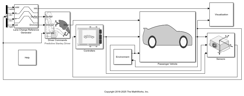
Run a Double-Lane Change Maneuver
1. Open the Lane Change Reference Generator block. By default, the maneuver is set with these parameters:
Longitudinal entrance velocity setpoint — 35 mph
Vehicle width — 2 m
Lateral reference position breakpoints and Lateral reference data — Values that specify the lateral reference trajectory as a function of the longitudinal distance
2. In the Visualization subsystem, open the 3D Engine block. By default, the 3D Engine parameter is set to Disabled. Simulating models in the 3D visualization environment requires Simulink® 3D Animation™. For the 3D visualization engine platform requirements and hardware recommendations, see the Unreal Engine Simulation Environment Requirements and Limitations.
3. Run the maneuver. As the simulation runs, view the vehicle information.
mdl = 'DLCReferenceApplication';
sim(mdl);
### Searching for referenced models in model 'DLCReferenceApplication'.
### Total of 3 models to build.
### Starting serial model build.
### Successfully updated the model reference simulation target for: Driveline
### Successfully updated the model reference simulation target for: PassVeh14DOF
### Successfully updated the model reference simulation target for: SiMappedEngineV

Build Summary

Model reference simulation targets:

Model            Build Reason                                        Status                        Build Duration
=================================================================================================================
Driveline        Target (Driveline_msf.mexw64) did not exist.        Code generated and compiled.  0h 0m 27.52s
PassVeh14DOF     Target (PassVeh14DOF_msf.mexw64) did not exist.     Code generated and compiled.  0h 1m 46.001s
SiMappedEngineV  Target (SiMappedEngineV_msf.mexw64) did not exist.  Code generated and compiled.  0h 0m 16.022s

3 of 3 models built (0 models already up to date)
Build duration: 0h 2m 35.446s
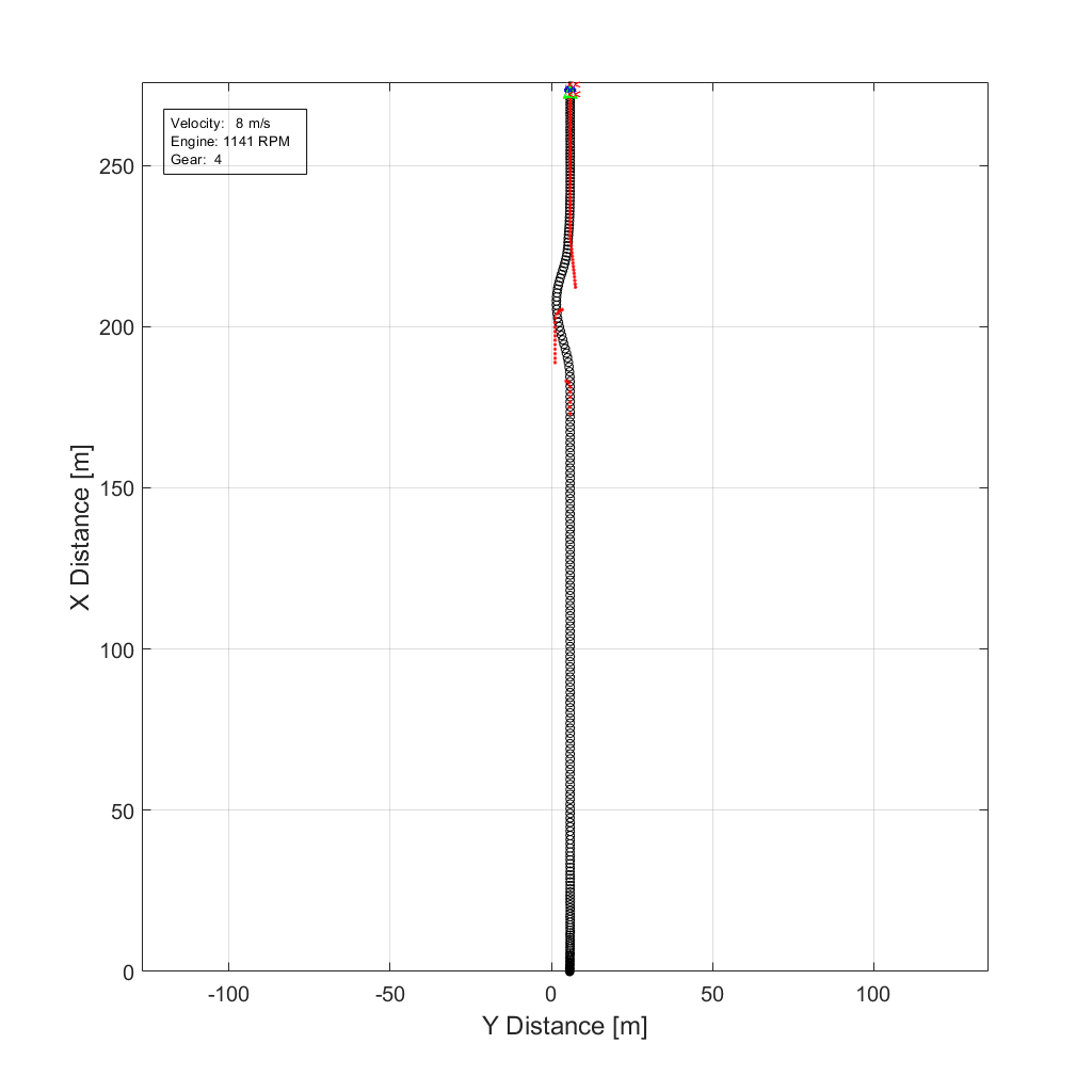
In the Vehicle Position window, view the vehicle longitudinal distance as a function or the lateral distance.
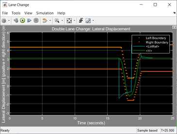
In the Visualization subsystem, open the Lane Change scope block to display the lateral displacement as a function of time. The red and orange lines mark the cone boundaries. The blue line marks the reference trajectory and the green line marks the actual trajectory. The green line does come close to the red line that marks the cones.
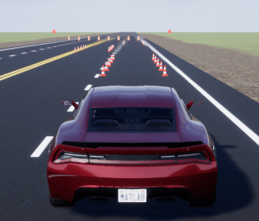
In the Visualization subsystem, if you enable the 3D Engine block visualization environment, you can view the vehicle response in the
AutoVrtlEnvwindow.
Sweep Surface Friction
Run the reference application on three road surfaces with different friction scaling coefficients. Use the results to analyze the yaw stability and help determine the success of the maneuver.
1. In the double-lane change reference application model DLCReferenceApplication, open the Environment subsystem. The Friction block parameter Constant value specifies the friction scaling coefficient. By default, the friction scaling coefficient is 1.0. The reference application uses the coefficient to adjust the friction at every time step.
2. Enable signal logging for the velocity, lane, and ISO signals. You can use the Simulink® editor or, alternatively, these MATLAB® commands. Save the model.
Enable signal logging for the Lane Change Reference Generator outport Lane signal.
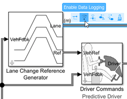
mdl = 'DLCReferenceApplication';
ph=get_param('DLCReferenceApplication/Lane Change Reference Generator','PortHandles');
set_param(ph.Outport(1),'DataLogging','on');
Enable signal logging for the Passenger Vehicle block outport signal.
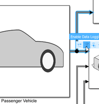
ph=get_param('DLCReferenceApplication/Passenger Vehicle','PortHandles');
set_param(ph.Outport(1),'DataLogging','on');
In the Visualization subsystem, enable signal logging for the ISO block.
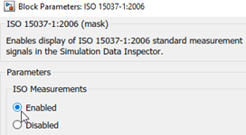
set_param([mdl '/Visualization/ISO 15037-1:2006'],'Measurement','Enable');
3. Set up a vector with the friction scaling coefficients, lambdamu, that you want to investigate. For example, to examine friction scaling coefficients equal to 0.9, 0.95, and 1.0, at the command line enter:
lambdamu = [0.9, 0.95, 1.0];
numExperiments = length(lambdamu);
4. Create an array of simulation inputs that sets lambdamu equal to the Friction constant block parameter.
for idx = numExperiments:-1:1
    in(idx) = Simulink.SimulationInput(mdl);
    in(idx) = in(idx).setBlockParameter([mdl '/Environment/Friction'],...
        'Value',['ones(4,1).*',num2str(lambdamu(idx))]);
end
5. Set the simulation stop time at 25 s. Save the model and run the simulations. If available, use parallel computing.
set_param(mdl,'StopTime','25')
save_system(mdl)
tic;
simout = parsim(in,'ShowSimulationManager','on');
toc;
[27-Dec-2024 11:21:09] Checking for availability of parallel pool...
[27-Dec-2024 11:21:09] Starting Simulink on parallel workers...
[27-Dec-2024 11:21:12] Loading project on parallel workers...
[27-Dec-2024 11:21:12] Configuring simulation cache folder on parallel workers...
[27-Dec-2024 11:21:12] Loading model on parallel workers...
[27-Dec-2024 11:21:35] Running simulations...
[27-Dec-2024 11:22:32] Completed 1 of 3 simulation runs
[27-Dec-2024 11:22:32] Received simulation output (size: 11.97 MB) for run 3 from parallel worker.
[27-Dec-2024 11:22:56] Completed 2 of 3 simulation runs
[27-Dec-2024 11:22:56] Received simulation output (size: 12.96 MB) for run 2 from parallel worker.
[27-Dec-2024 11:23:26] Completed 3 of 3 simulation runs
[27-Dec-2024 11:23:26] Received simulation output (size: 14.15 MB) for run 1 from parallel worker.
[27-Dec-2024 11:23:26] Cleaning up parallel workers...
Elapsed time is 150.337127 seconds.
6. After the simulations complete, close the Simulation Data Inspector windows.
Use Simulation Data Inspector to Analyze Results
Use the Simulation Data Inspector to examine the results. You can use the UI or, alternatively, command-line functions.
1. Open the Simulation Data Inspector. On the Simulink Toolstrip, on the Simulation tab, under Review Results, click Data Inspector.
In the Simulation Data Inspector, select Import.
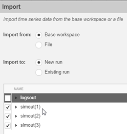
In the Import dialog box, clear
logsout. Selectsimout(1),simout(2), andsimout(3). Select Import.
Use the Simulation Data Inspector to examine the results.
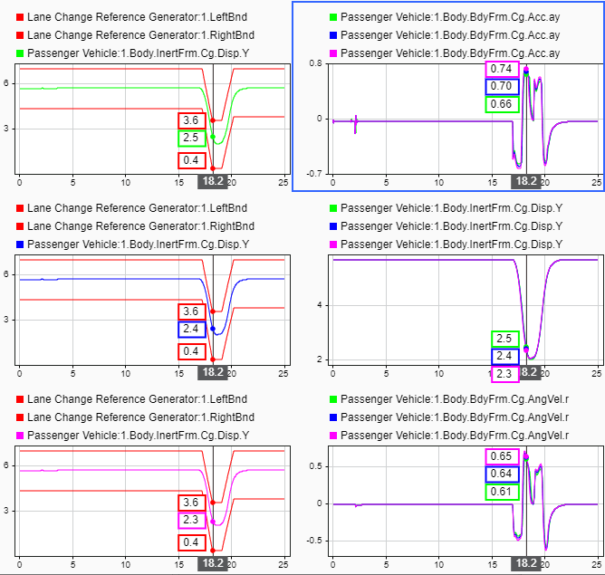
2. Alternatively, use these MATLAB commands to create 6 plots. The first three plots mark the upper lane boundary, UB, lower lane boundary, LB, and lateral vehicle distance, Y, for each run.
The next three plots provide the lateral acceleration, ay, lateral vehicle distance, Y, and yaw rate, r, for each run.
for idx = 1:numExperiments
    % Create sdi run object
    simoutRun(idx)=Simulink.sdi.Run.create;
    simoutRun(idx).Name=['lambdamu = ', num2str(lambdamu(idx))];
    add(simoutRun(idx),'vars',simout(idx));
end
sigcolor=[1 0 0];
for idx = 1:numExperiments
    % Extract the maneuver upper and lower lane boundaries
    ubsignal(idx)=getSignalsByName(simoutRun(idx), 'Lane Change Reference Generator:1.LeftBnd');
    ubsignal(idx).LineColor = sigcolor;
    lbsignal(idx)=getSignalsByName(simoutRun(idx), 'Lane Change Reference Generator:1.RightBnd');
    lbsignal(idx).LineColor = sigcolor;
end
sigcolor=[0 1 0;0 0 1;1 0 1];
for idx = 1:numExperiments
    % Extract the lateral acceleration, position, and yaw rate
    ysignal(idx)=getSignalsByName(simoutRun(idx), 'Passenger Vehicle:1.Body.InertFrm.Cg.Disp.Y');
    ysignal(idx).LineColor =sigcolor((idx),:);
    rsignal(idx)=getSignalsByName(simoutRun(idx), 'Passenger Vehicle:1.Body.BdyFrm.Cg.AngVel.r');
    rsignal(idx).LineColor =sigcolor((idx),:);
    asignal(idx)=getSignalsByName(simoutRun(idx), 'Passenger Vehicle:1.Body.BdyFrm.Cg.Acc.ay');
    asignal(idx).LineColor =sigcolor((idx),:);
end
Simulink.sdi.view
Simulink.sdi.setSubPlotLayout(numExperiments,2);
for idx = 1:numExperiments
    %  Plot the lateral position and lane boundaries
    plotOnSubPlot(ubsignal(idx),(idx),1,true);
    plotOnSubPlot(lbsignal(idx),(idx),1,true);
    plotOnSubPlot(ysignal(idx),(idx),1,true);
end
for idx = 1:numExperiments
    % Plot the lateral acceleration, position, and yaw rate
    plotOnSubPlot(asignal(idx),1,2,true);
    plotOnSubPlot(ysignal(idx),2,2,true);
    plotOnSubPlot(rsignal(idx),3,2,true);
end
The results are similar to these plots, which indicate that the vehicle has a yaw rate of about .66 rad/s when the friction scaling coefficient is equal to 1.
Further Analysis
To explore the results further, use these commands to extract the lateral acceleration, steering angle, and vehicle trajectory from the simout object.
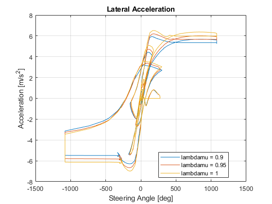
1. Extract the lateral acceleration and steering angle. Plot the data. The results are similar to this plot. They indicate that the greatest lateral acceleration occurs when the friction scaling coefficient is 1.
figure
for idx = 1:numExperiments
    % Extract Data
    log = get(simout(idx),'logsout');
    sa=log.get('Steering-wheel angle').Values;
    ay=log.get('Lateral acceleration').Values;
    legend_labels{idx} = ['lambdamu = ', num2str(lambdamu(idx))];
    % Plot steering angle vs. lateral acceleration
    plot(sa.Data,ay.Data)
    hold on
end
% Add labels to the plots
legend(legend_labels, 'Location', 'best');
title('Lateral Acceleration')
xlabel('Steering Angle [deg]')
ylabel('Acceleration [m/s^2]')
grid on
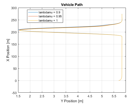
2. Extract the vehicle path. Plot the data. The results are similar to this plot. They indicate that the greatest lateral vehicle position occurs when the friction scaling coefficient is 0.9.
figure
for idx = 1:numExperiments
    % Extract Data
    log = get(simout(idx),'logsout');
    xValues = getSignalsByName(simoutRun(idx), 'Passenger Vehicle:1.Body.InertFrm.Cg.Disp.X').Values;
    yValues = getSignalsByName(simoutRun(idx), 'Passenger Vehicle:1.Body.InertFrm.Cg.Disp.Y').Values;
    x = xValues.Data;
    y = yValues.Data;
    legend_labels{idx} = ['lambdamu = ', num2str(lambdamu(idx))];
    % Plot vehicle location
    plot(y,x)
    hold on
end
% Add labels to the plots
legend(legend_labels, 'Location', 'best');
title('Vehicle Path')
xlabel('Y Position [m]')
ylabel('X Position [m]')
grid on

See Also
Simulink.SimulationInput | Simulink.SimulationOutput
References
[1] ISO 3888-2: 2011. Passenger cars — Test track for a severe lane-change manoeuvre.