Tangent Plane and Normal Line of Implicit Surface
Since R2021b
This example shows how to find the tangent plane and the normal line of an implicit surface. This example uses symbolic matrix variables (with the symmatrix data type) for compact mathematical notation.
A surface can be defined implicitly, such as the sphere . In general, an implicitly defined surface is expressed by the equation . This example finds the tangent plane and the normal line of a sphere with radius .
Create a symbolic matrix variable to represent the coordinates. Define the spherical function as .
clear; close all; clc
syms r [1 3] matrix
f = r*r.'
f =
The implicit equation represents a sphere. Convert the equation to the syms data type using symmatrix2sym. Plot the equation by using the fimplicit3 function.
feqn = symmatrix2sym(f == 14)
feqn =
fimplicit3(feqn)
axis equal
axis([-6 6 -6 6 -6 6])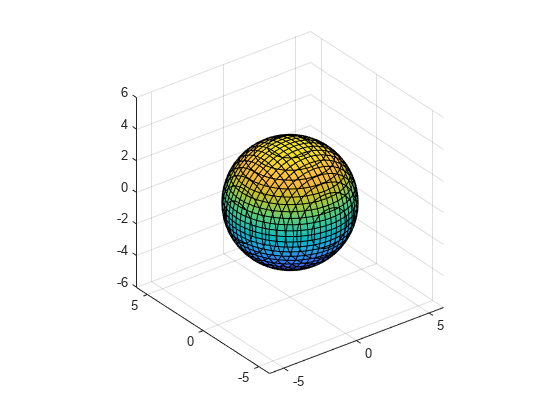
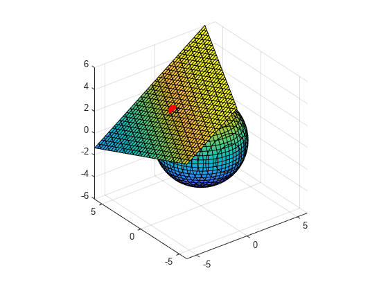
Next, find the tangent plane and normal line at the point .
Recall that the gradient vector of is . The equation for the tangent plane at the point is then given by . In compact mathematical notation, the tangent plane equation can be written as .
Find the gradient of using the gradient function. Note that the result is a 3-by-1 symbolic matrix variable.
fgrad = gradient(f,r)
fgrad =
size(fgrad)
ans = 1×2

     3     1
Define the equation for the tangent plane. Use the subs function to evaluate the gradient at the point .
r0 = [-2,1,3];
fplane = (r-r0)*subs(fgrad,r,r0)
fplane =
Plot the point using plot3, and plot the tangent plane using fimplicit3.
hold on
plot3(r0(1),r0(2),r0(3),'ro',MarkerSize = 10,MarkerFaceColor = 'r')
fimplicit3(symmatrix2sym(fplane == 0))
The equation for the normal line at the point is given by . In compact mathematical notation, the equation can be written as .
Define the equation for the normal line.
syms t
n = r0 + t*subs(fgrad,r,r0).'
n =
Convert the normal line equation to the syms data type using symmatrix2sym. Extract the parametric curves , , and for the normal line by indexing into n. Plot the normal line using fplot3.
n = symmatrix2sym(n)
n =
fplot3(n(1),n(2),n(3),[0 1],'r->')