Analyze and Manipulate Differential Algebraic Equations
This example shows how to solve differential algebraic equations (DAEs) of high differential index using Symbolic Math Toolbox™.
Engineers often specify the behavior of their physical objects (mechanical systems, electrical devices, and so on) by a mixture of differential equations and algebraic equations. MATLAB® provides special numerical solvers, such as ode15i and ode15s, capable of integrating such DAEs — provided that their differential index does not exceed 1.
This example shows the workflow from setting up the model as a system of differential equations with algebraic constraints to the numerical simulation. The following Symbolic Math Toolbox functions are used.
daeFunctionfindDecoupledBlocksincidenceMatrixisOfLowDAEIndexreduceDifferentialOrdermassMatrixFormreduceDAEIndexreduceDAEToODEreduceRedundanciessym/decic
Define Parameters of the Model
Consider a 2-D physical pendulum, consisting of a mass m attached to the origin by a string of constant length r. Only the gravitational acceleration g = 9.81 m/s^2 acts on the mass. The model consists of second-order differential equation for the position (x(t), y(t)) of the mass with an unknown force F(t) inside the string which serves for keeping the mass on the circle. The force is directed along the string.
syms x(t) y(t) F(t) m g r
eqs = [m*diff(x(t),t,t) == F(t)/r*x(t);
       m*diff(y(t),t,t) == F(t)/r*y(t) - m*g;
       x(t)^2 + y(t)^2 == r^2]
eqs =
vars = [x(t),y(t),F(t)]
vars =
Rewrite this DAE system to a system of first-order differential algebraic equations.
[eqs,vars,newVars] = reduceDifferentialOrder(eqs,vars)
eqs =
vars =
newVars =
Try Solving the High-Index DAE System
Before you can use a numerical MATLAB solver, such as ode15i, you must follow these steps.
Convert the system of DAEs to a MATLAB function handle.
Choose numerical values for symbolic parameters of the system.
Set consistent initial conditions.
To convert a DAE system to a MATLAB function handle, use daeFunction.
F = daeFunction(eqs,vars,[m g r])
F = function_handle with value:
    @(t,in2,in3,in4)[in3(4,:).*in4(:,1)-(in2(3,:).*in2(1,:))./in4(:,3);in3(5,:).*in4(:,1)+in4(:,1).*in4(:,2)-(in2(3,:).*in2(2,:))./in4(:,3);-in4(:,3).^2+in2(1,:).^2+in2(2,:).^2;in2(4,:)-in3(1,:);in2(5,:)-in3(2,:)]
Assign numerical values to the symbolic parameters of the system: m = 1kg, g = 9.18m/s^2, and r = 1m.
f = @(t,y,yp) F(t,y,yp,[1 9.81 1])
f = function_handle with value:
    @(t,y,yp)F(t,y,yp,[1,9.81,1])
The function handle f is a suitable input for the numerical solver ode15i. The next step is to compute consistent initial conditions. Use odeset to set numerical tolerances. Then use the MATLAB decic function to compute consistent initial conditions y0, yp0 for the positions and the derivatives at time t0 = 0.
opt = odeset(RelTol=1e-4,AbsTol=1e-4);
t0 = 0;
[y0,yp0] = decic(f,t0,[0.98;-0.21;zeros(3,1)],[],zeros(5,1),[],opt)
y0 = 5×1

    0.9777
   -0.2100
         0
         0
         0
yp0 = 5×1

         0
         0
         0
         0
   -9.8100
Test the initial conditions:
f(t0, y0, yp0)
ans = 5×1
10-16 ×

         0
         0
   -0.3469
         0
         0
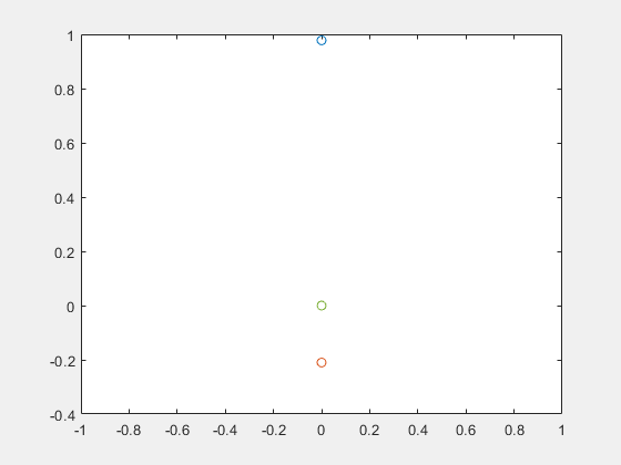
Now you can use ode15i to try solving the system. When you call ode15i, the integration stops immediately and issues the following warnings.
Warning: Matrix is singular, close to singular or badly scaled.
Results may be inaccurate. RCOND = NaN.
Warning: Failure at t=0.000000e+00.
Unable to meet integration tolerances without reducing the step
size below the smallest value allowed (0.000000e+00) at time t.
For this example, ode15i issues these warnings multiple times. For readability, disable warnings by using warning("off","all") before calling ode15i and then enable them again.
tfinal = 0.5;
s = warning("off","all");
ode15i(f,[t0,tfinal],y0,yp0,opt);
warning(s)
Analyze and Adjust the DAE System
Check the differential index of the DAE system.
isLowIndexDAE(eqs,vars)
ans = logical
   0
This result explains why ode15i cannot solve this system. This function requires the input DAE system to be of differential index 0 or 1. Reduce the differential index by extending the model to an equivalent larger DAE system that includes some hidden algebraic constraints.
[eqs,vars newVars,index] = reduceDAEIndex(eqs,vars)
eqs =
vars =
newVars =
index =
3
The fourth output shows that the differential index of the original model is three. Simplify the new system.
[eqs,vars,S] = reduceRedundancies(eqs,vars)
eqs =
vars =
S = struct with fields:
      solvedEquations: [3×1 sym]
    constantVariables: [0×2 sym]
    replacedVariables: [3×2 sym]
       otherEquations: [0×1 sym]
Check if the new system has a low differential index (0 or 1).
isLowIndexDAE(eqs,vars)
ans = logical
   1
Solve the Low-Index DAE System
Generate a MATLAB function handle that replaces the symbolic parameters by numerical values.
F = daeFunction(eqs,vars,[m g r])
F = function_handle with value:
    @(t,in2,in3,in4)[-(in2(3,:).*in2(1,:)-in2(7,:).*in4(:,1).*in4(:,3))./in4(:,3);(-in2(3,:).*in2(2,:)+in2(6,:).*in4(:,1).*in4(:,3)+in4(:,1).*in4(:,2).*in4(:,3))./in4(:,3);-in4(:,3).^2+in2(1,:).^2+in2(2,:).^2;in2(4,:).*in2(1,:).*2.0+in2(5,:).*in2(2,:).*2.0;in2(7,:).*in2(1,:).*2.0+in2(6,:).*in2(2,:).*2.0+in2(4,:).^2.*2.0+in2(5,:).^2.*2.0;in2(6,:)-in3(5,:);in2(5,:)-in3(2,:)]
f = @(t,y,yp) F(t,y,yp,[1 9.81 1])
f = function_handle with value:
    @(t,y,yp)F(t,y,yp,[1,9.81,1])
Compute consistent initial conditions for the index reduced by the MATLAB decic function. Here, opt is the options structure that sets numerical tolerances. You already computed it using odeset.
[y0,yp0] = decic(f,t0,[0.98;-0.21;zeros(5,1)],[],zeros(7,1),[],opt)
y0 = 7×1

    0.9779
   -0.2093
   -2.0528
    0.0000
         0
   -9.3804
   -2.0074
yp0 = 7×1

         0
         0
         0
         0
   -9.3804
         0
         0
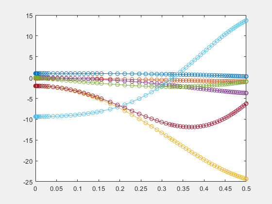
Solve the system and plot the solution.
ode15i(f,[t0 tfinal],y0,yp0,opt)