stepwise
Interactive stepwise regression
Syntax
stepwise

stepwise(X,y)

stepwise(X,y,inmodel,penter,premove)
Description
stepwise uses the sample
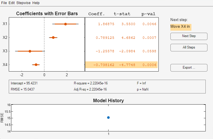
data in hald.mat to display a graphical user interface
for performing stepwise regression of the response values in heat on
the predictive terms in ingredients.

The upper left of the interface displays estimates of the coefficients for all potential terms, with horizontal bars indicating 90% (colored) and 95% (grey) confidence intervals. The red color indicates that, initially, the terms are not in the model. Values displayed in the table are those that would result if the terms were added to the model.
The middle portion of the interface displays summary statistics for the entire model. These statistics are updated with each step.
The lower portion of the interface, Model History, displays the RMSE for the model. The plot tracks the RMSE from step to step, so you can compare the optimality of different models. Hover over the blue dots in the history to see which terms were in the model at a particular step. Click on a blue dot in the history to open a copy of the interface initialized with the terms in the model at that step.
Initial models, as well as entrance/exit tolerances for the p-values
of F-statistics, are specified using additional
input arguments to stepwise. Defaults are an
initial model with no terms, an entrance tolerance of 0.05, and an
exit tolerance of 0.10.
To center and scale the input data (compute z-scores)
to improve conditioning of the underlying least-squares problem, select Scale
Inputs from the Stepwise menu.
You proceed through a stepwise regression in one of two ways:
Click Next Step to select the recommended next step. The recommended next step either adds the most significant term or removes the least significant term. When the regression reaches a local minimum of RMSE, the recommended next step is “Move no terms.” You can perform all of the recommended steps at once by clicking All Steps.
Click a line in the plot or in the table to toggle the state of the corresponding term. Clicking a red line, corresponding to a term not currently in the model, adds the term to the model and changes the line to blue. Clicking a blue line, corresponding to a term currently in the model, removes the term from the model and changes the line to red.
To call addedvarplot and
produce an added variable plot from the stepwise interface,
select Added Variable Plot from the Stepwise menu.
A list of terms is displayed. Select the term you want to add, and
then click OK.
Click Export to display a dialog box that allows you to select information from the interface to save to the MATLAB® workspace. Check the information you want to export and, optionally, change the names of the workspace variables to be created. Click OK to export the information.
stepwise(X,y) displays the
interface using the p predictive terms in the n-by-p matrix X and
the response values in the n-by-1 vector y.
Distinct predictive terms should appear in different columns of X.
Note
stepwise automatically includes a constant
term in all models. Do not enter a column of 1s directly into X.
stepwise treats NaN values
in either X or y as missing
values, and ignores them.
stepwise(X,y,inmodel,penter,premove) additionally
specifies the initial model (inmodel) and the
entrance (penter) and exit (premove)
tolerances for the p-values of F-statistics. inmodel is
either a logical vector with length equal to the number of columns
of X, or a vector of indices, with values ranging
from 1 to the number of columns in X. The value
of penter must be less than or equal to the value
of premove.
Algorithms
Stepwise regression is a systematic method for adding and removing terms from a multilinear model based on their statistical significance in a regression. The method begins with an initial model and then compares the explanatory power of incrementally larger and smaller models. At each step, the p value of an F-statistic is computed to test models with and without a potential term. If a term is not currently in the model, the null hypothesis is that the term would have a zero coefficient if added to the model. If there is sufficient evidence to reject the null hypothesis, the term is added to the model. Conversely, if a term is currently in the model, the null hypothesis is that the term has a zero coefficient. If there is insufficient evidence to reject the null hypothesis, the term is removed from the model. The method proceeds as follows:
Fit the initial model.
If any terms not in the model have p-values less than an entrance tolerance (that is, if it is unlikely that they would have zero coefficient if added to the model), add the one with the smallest p value and repeat this step; otherwise, go to step 3.
If any terms in the model have p-values greater than an exit tolerance (that is, if it is unlikely that the hypothesis of a zero coefficient can be rejected), remove the one with the largest p value and go to step 2; otherwise, end.
Depending on the terms included in the initial model and the order in which terms are moved in and out, the method may build different models from the same set of potential terms. The method terminates when no single step improves the model. There is no guarantee, however, that a different initial model or a different sequence of steps will not lead to a better fit. In this sense, stepwise models are locally optimal, but may not be globally optimal.
Version History
Introduced before R2006a