Negative Binomial Distribution
Definition
The negative binomial pdf is
for x ≥ 0, where q = 1 – p. The probability y is zero when x is not an integer.
When r is not an integer, the binomial coefficient in the definition of the pdf is replaced by the equivalent expression
Background
In its simplest form (when r is an integer), the negative binomial distribution models the number of failures x before a specified number of successes is reached in a series of independent, identical trials. Its parameters are the probability of success in a single trial, p, and the number of successes, r. A special case of the negative binomial distribution, when r = 1, is the geometric distribution, which models the number of failures before the first success.
More generally, r can take on non-integer values. This form of the negative binomial distribution has no interpretation in terms of repeated trials, but, like the Poisson distribution, it is useful in modeling count data. The negative binomial distribution is more general than the Poisson distribution because it has a variance that is greater than its mean, making it suitable for count data that do not meet the assumptions of the Poisson distribution. In the limit, as r increases to infinity, the negative binomial distribution approaches the Poisson distribution.
Parameters
The negative binomial distribution uses the following parameters.
| Parameter | Description | Support |
|---|---|---|
| r | Number of successes | |
| p | Probability of success |
Negative Binomial Distribution Parameters
Determine the parameters of a negative binomial distribution.
Suppose you are collecting data on the number of auto accidents on a busy highway, and would like to be able to model the number of accidents per day. Because these are count data, and because there are a very large number of cars and a small probability of an accident for any specific car, you might think to use the Poisson distribution. However, the probability of having an accident is likely to vary from day to day as the weather and amount of traffic change, and so the assumptions needed for the Poisson distribution are not met. In particular, the variance of this type of count data sometimes exceeds the mean by a large amount. The data below exhibit this effect: most days have few or no accidents, and a few days have a large number.
accident = [2  3  4  2  3  1  12  8  14  31  23  1  10  7  0];
m = mean(accident)
m =
8.0667
v = var(accident)
v =
79.3524
The negative binomial distribution is more general than the Poisson, and is often suitable for count data when the Poisson is not. The function nbinfit returns the maximum likelihood estimates (MLEs) and confidence intervals for the parameters of the negative binomial distribution. Observe the results from fitting the accident data.
[phat,pci] = nbinfit(accident)
phat = 1×2

    1.0060    0.1109
pci = 2×2

    0.2152    0.0171
    1.7968    0.2046
It is difficult to give a physical interpretation in this case to the individual parameters. However, the estimated parameters can be used in a model for the number of daily accidents. For example, a plot of the estimated cumulative probability function shows that while there is an estimated 10% chance of no accidents on a given day, there is also about a 10% chance that there will be 20 or more accidents.
plot(0:50,nbincdf(0:50,phat(1),phat(2)),".-");
xlabel("Accidents per Day")
ylabel("Cumulative Probability")

Example
Compute and Plot Negative Binomial Distribution pdf
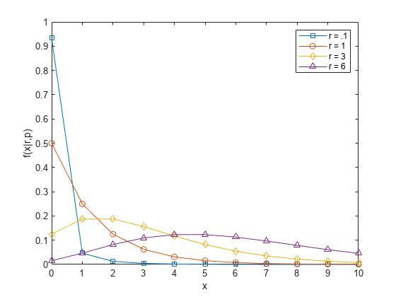
Compute and plot the pdf using four different values for the parameter r, the desired number of successes: .1, 1, 3, and 6. In each case, the probability of success p is .5.
x = 0:10;
plot(x,nbinpdf(x,.1,.5),'s-', ...
     x,nbinpdf(x,1,.5),'o-', ...
     x,nbinpdf(x,3,.5),'d-', ...
     x,nbinpdf(x,6,.5),'^-');
legend({'r = .1' 'r = 1' 'r = 3' 'r = 6'})
xlabel('x')
ylabel('f(x|r,p)')

The plot shows that the negative binomial distribution can take on a variety of shapes, ranging from very skewed to nearly symmetric, depending on the value of r.